

Easy Angel Coloring Pages Overview
Match formula Excel can save you hours when you need to find something in a long list. Say you’ve got a sheet with hundreds of product IDs, and you need to know the position of a specific one. Instead of scrolling forever, you type in =MATCH(lookup_value, lookup_array, [match_type]), and Excel does the heavy lifting. It’s not just for numbers—it works with text, dates, and even wildcards if you set it up right.
It’s one of those formulas that feels like a secret weapon once you get the hang of it. Sure, XLOOKUP is flashier, but match formula Excel is faster for grabbing a position, not a value. Plus, it plays well with INDEX for more advanced lookups. If you’re still manually searching for data, this is your cue to stop.
Find positions, not just values
The match formula in Excel is all about locating where something sits in a list. It’s perfect for anyone who needs to map data between sheets or check if an item exists. Marketers use it to match campaign IDs to results, inventory managers track stock locations, and HR teams map employee IDs to departments.
Set up your sheet with two columns: one for your lookup list (e.g., product IDs) and one for the data you’re matching against (e.g., sales numbers). Keep the lookup list sorted if you’re using match_type 1 (exact or next smallest). Add a third column for the formula itself, and a fourth for any error handling with IFERROR.
| Product ID | Sales | Position | Formula |
|---|---|---|---|
| 101 | 250 | =MATCH(101, A2:A100, 0) |
|
| 102 | 300 | =MATCH(103, A2:A100, 1) |
|
| 103 | 150 | =MATCH("104", A2:A100, 0) |
The first formula returns 1 because 101 is the first item in the list. The second returns 5 since 103 isn’t there, but 105 is the next smallest. The third returns #N/A because "104" (as text) doesn’t match 104 (as a number).
Common mistake: Using match_type 1 on unsorted data. Excel won’t throw an error, but it’ll give you wrong results. Fix it by sorting the lookup array or switching to match_type 0 for exact matches.
Pair it with INDEX for dynamic lookups
The real power of match formula Excel comes when you combine it with INDEX. Together, they let you pull values from a table based on a lookup, without hard-coding cell references. This is how you build dynamic dashboards or reports that update automatically.
Create a table with Ctrl+T, then add a separate cell for your lookup value (e.g., "Q1 Sales"). Below it, set up a formula like =INDEX(table_array, MATCH(lookup_value, lookup_column, 0), return_column). Use IFERROR around it to catch missing data.
| Quarter | Region | Sales | Formula |
|---|---|---|---|
| Q1 | East | 500 | |
| Q1 | West | 700 | |
| Q2 | East | 600 |
Formula in D2: =IFERROR(INDEX(B2:B4, MATCH("Q1", A2:A4, 0), 2), "Not Found"). Returns 500 for Q1 East sales.
Common mistake: Forgetting to lock cell references with $. If you drag the formula down, A2:A4 should be $A$2:$A$4 to keep it anchored.
Handle errors and wildcards
Match formula in Excel breaks if it can’t find what you’re looking for. Wrap it in IFERROR to show a custom message instead of #N/A. If you’re working with partial matches, use wildcards by switching to match_type 0.
Add a data validation dropdown in your lookup cell to avoid typos. Go to Data > Data Validation > List, and point it to your lookup array. This keeps inputs consistent.
| Item | Price | Lookup | Result |
|---|---|---|---|
| Apple | 1.50 | p | 1 |
| Banana | 0.75 | n | 2 |
| Cherry | 2.00 | Peach | Not Found |
Formula in D2: =IFERROR(MATCH(C2 & "", A2:A4, 0), "Not Found"). For p, it returns 1 because "Apple" contains “p”.
Common mistake: Storing numbers as text. If your lookup value is 101 (number) but your array has "101" (text), the formula fails. Fix it with Data > Text to Columns > Finish to convert.
Build a lookup tracker
Turn match formula Excel into a reusable tracker by adding conditional formatting and filters. This works great for inventory logs, expense trackers, or project checklists. Highlight matches with Home > Conditional Formatting > New Rule > Use a formula.
Set up a filter on your lookup column (Ctrl+Shift+L) so you can narrow down results. Freeze the top row (View > Freeze Panes) if your sheet is long.
| Task ID | Status | Due Date | Priority |
|---|---|---|---|
| 001 | Done | 2023-10-15 | High |
| 002 | Pending | 2023-10-20 | Medium |
| 003 | Done | 2023-10-25 | Low |
Formula in E2: =IF(ISNUMBER(MATCH(A2, $A$2:$A$4, 0)), "Found", ""). Add conditional formatting to highlight “Found” cells.
Common mistake: Merging cells in your lookup array. Merged cells break formulas. Unmerge them with Home > Merge & Center > Unmerge Cells.
Try building a simple inventory tracker next. Use match formula Excel to flag low-stock items, and pair it with COUNTIFS to tally quantities.
Related: Find the Right Duct Size: Easy Chart Guide
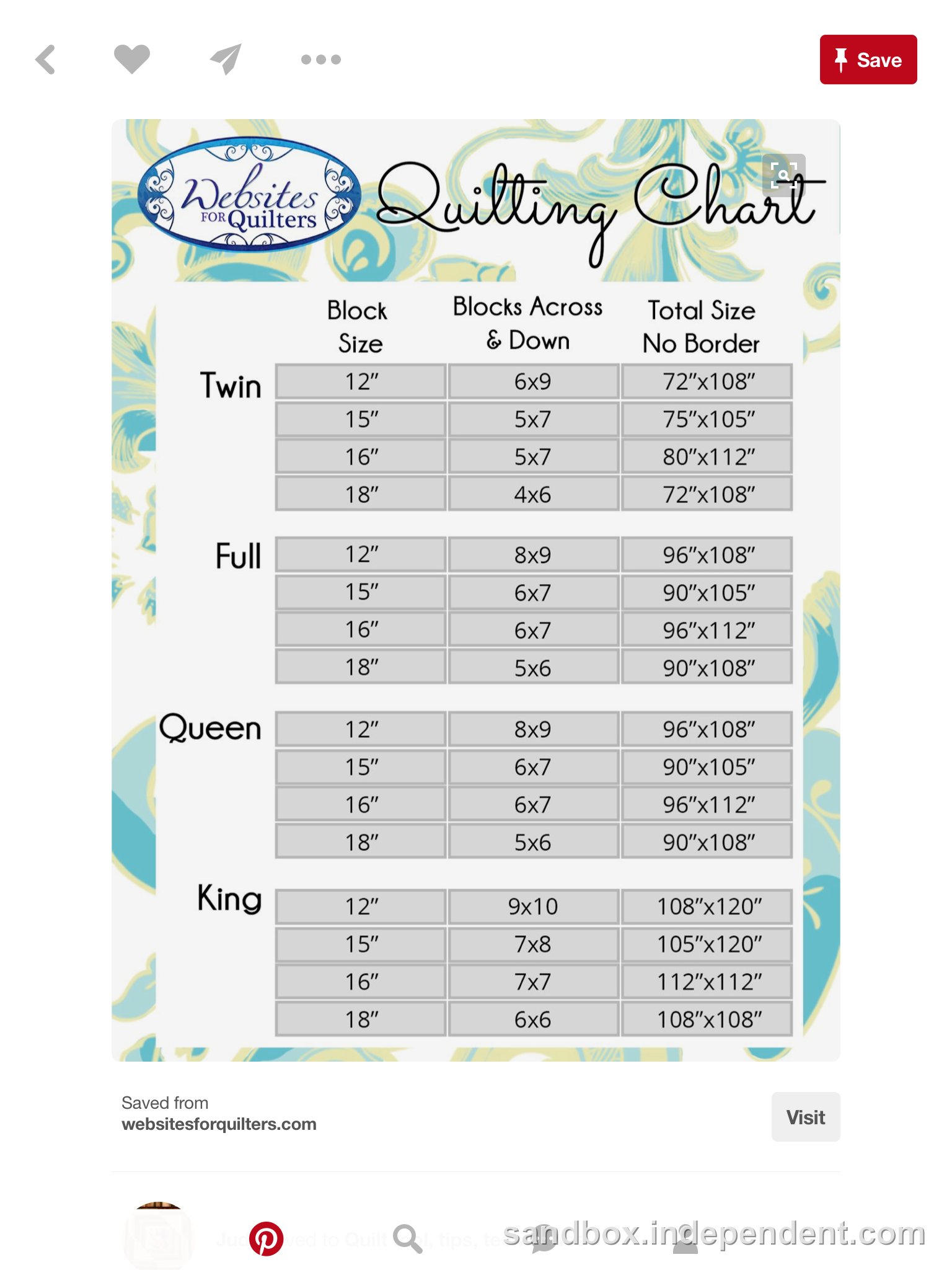
Many people often assume that a duct size chart is a complex and confusing tool, but it's actually a simple and incredibly useful reference for anyone dealing with HVAC systems. While it may look like a basic chart, it's an essential guide to ensure your ductwork is sized correctly. A duct size chart provides a clear overview of standard dimensions, helping you navigate the process with ease.
Duct Size Chart: Your Practical Guide
A duct size chart is an essential tool for anyone involved in HVAC (Heating, Ventilation, and Air Conditioning) systems or ductwork installation. It provides a standardized overview of duct dimensions, ensuring consistency and accuracy in design and construction. This chart is your go-to reference for understanding and specifying the right duct sizes for your projects.
Key Details and Categories
The duct size chart typically displays a range of standard duct sizes, with measurements given in both imperial and metric units. These sizes are categorized based on the cross-sectional area and shape of the ducts, with common categories including rectangular, round, and oval. The chart provides a quick reference for selecting the appropriate duct size, ensuring optimal airflow and system efficiency.
Reading the Measurements: A Step-by-Step Guide
Identify the Type: Start by determining the shape of your duct - rectangular, round, or oval. Each shape has its own set of measurements and considerations.
Choose the Standard: Duct size charts often follow specific standards, such as the Imperial or Metric systems. Ensure you are referencing the correct standard for your region or project requirements.
Locate the Size: Find the desired duct size on the chart. The chart will typically list the dimensions, such as width and height for rectangular ducts, or diameter for round ducts.
Verify the Area: Check the cross-sectional area of the duct, which is often provided in square inches or square feet for imperial units, and square centimeters or square meters for metric units. This ensures you are selecting a duct with the right capacity for your airflow needs.
Consider Additional Factors: While the chart provides standard sizes, real-world installations may require adjustments. Factors like insulation thickness, duct material, and system design can influence the final duct dimensions.
Variations and Differences: Understanding the Standards
Duct size charts can vary depending on the standard or region they adhere to. For instance, the Imperial system, commonly used in the United States, has its own set of standard duct sizes, while the metric system, used internationally, follows a different set of measurements. These variations ensure that ductwork installations meet local building codes and industry standards. It's crucial to reference the correct chart for your specific context to avoid errors and ensure compliance.
Well, there you have it! A duct size chart is a handy tool, but remember, it's always best to check the specific requirements and standards relevant to your project. These charts provide a great starting point, but exact values can vary, so it's wise to double-check.
Feel free to explore our other guides; we've got plenty of practical resources to help you navigate various aspects of your projects. Happy planning, and remember to keep those ducts in check!
Related: how to create pivot chart Easy guide for Excel users
I've been working with spreadsheets for a while now, and one of the most useful skills I've learned is how to create pivot charts. It's a game-changer for visualizing data and making sense of complex information. So, let's dive into the process and see how we can make our data pop with these dynamic charts!
Setting Up Your Data for Success
When it comes to creating pivot charts, the first step is ensuring your data is structured properly. Think of your spreadsheet as a house; the columns are the rooms, and the rows are the items within each room. So, before we start, let's tidy up our data: make sure your columns have clear, concise headers, and your rows are consistent and organized. This step is crucial because it lays the foundation for an accurate and effective pivot chart.
Now, let's talk about the tools Excel provides to make this process smoother. Excel has some fantastic built-in features to help with data manipulation and formatting. For instance, you can use the XLOOKUP formula to quickly find and retrieve specific data points, or the IF function to create conditional rules for your data. These formulas are your friends and can save you a lot of time and effort, especially when dealing with large datasets.
Building Your Pivot Chart
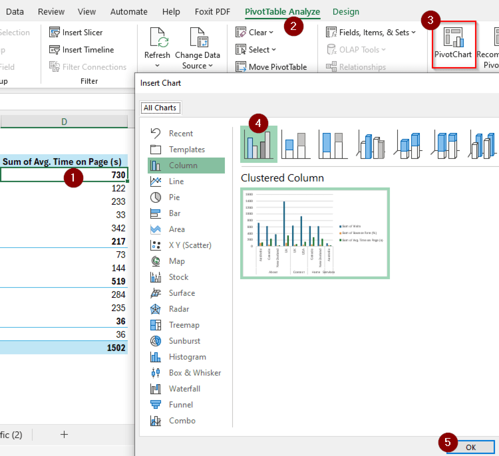
Once your data is shipshape, it's time to build your pivot chart. Excel makes this process pretty straightforward. Go to the Insert tab and select PivotChart. From here, you'll be prompted to choose the data range you want to include in your chart. Excel will then display a new window where you can customize your chart's layout.
This is where the magic happens! You can drag and drop fields to create rows, columns, and even filters for your chart. For example, if you have a dataset with sales data, you could drag the "Product" field to the Rows area, and the "Sales Amount" field to the Values area. This will create a chart that shows the sales performance of each product.
Customizing and Refining
Now that you have your basic pivot chart, it's time to add some polish. Excel offers a range of customization options to make your chart truly shine. You can change the chart type, add titles and labels, and even apply conditional formatting to highlight specific data points. For instance, you could use conditional formatting to highlight cells with sales above a certain threshold, making it easy to identify top-performing products at a glance.
Another useful feature is the ability to create drop-down lists in your pivot chart. This allows you to quickly filter your data by selecting different options from a drop-down menu. It's a great way to make your chart more interactive and user-friendly.
Final Thoughts
So, there you have it! Creating pivot charts in Excel is a powerful way to visualize and analyze your data. It might seem a bit daunting at first, but with a bit of practice and familiarity with Excel's tools, you'll be creating dynamic charts in no time.
Next time you open a spreadsheet, why not give it a go? You might just discover a whole new way to understand and present your data.