
Excel Invoice Template Vlookup Overview
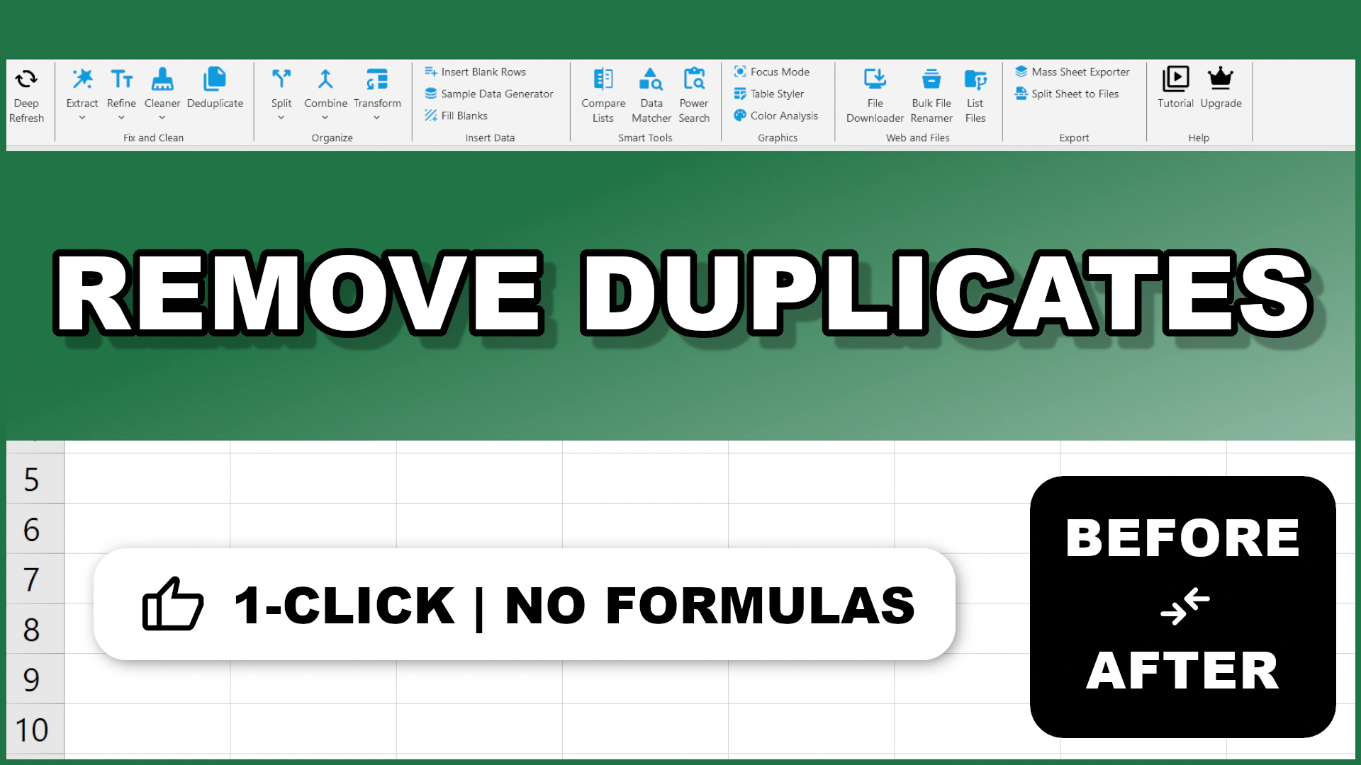
Ugh, duplicates in Excel. We've all been there, staring at a massive spreadsheet with rows and rows of data, only to realize there are multiple entries for the same thing. Remove duplicates Excel to the rescue! Let's get into how this handy feature works and why it's a lifesaver for anyone dealing with data.
So, you've got your Excel sheet open, and it's a mess of similar entries. Maybe it's a list of contacts, products, or sales data, and you need to clean it up. The "Remove Duplicates" feature is like a magic wand, but it's not as simple as clicking a button. You've got to set it up right to get the results you need.
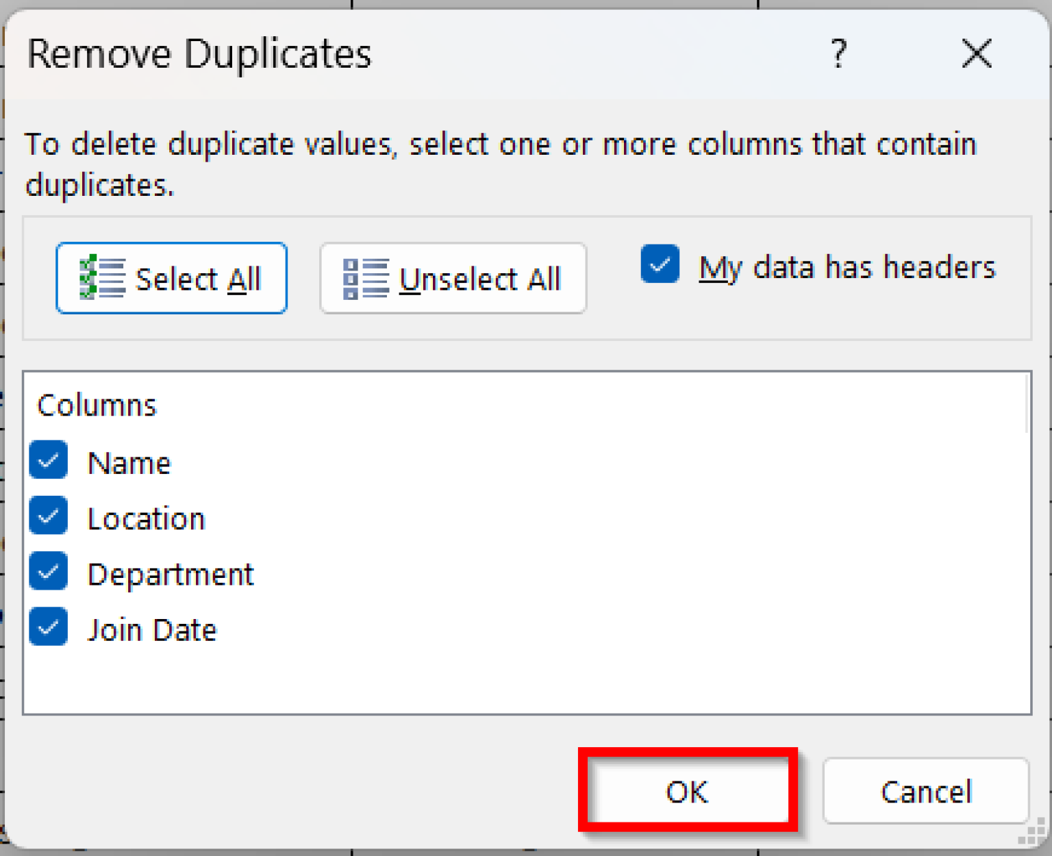
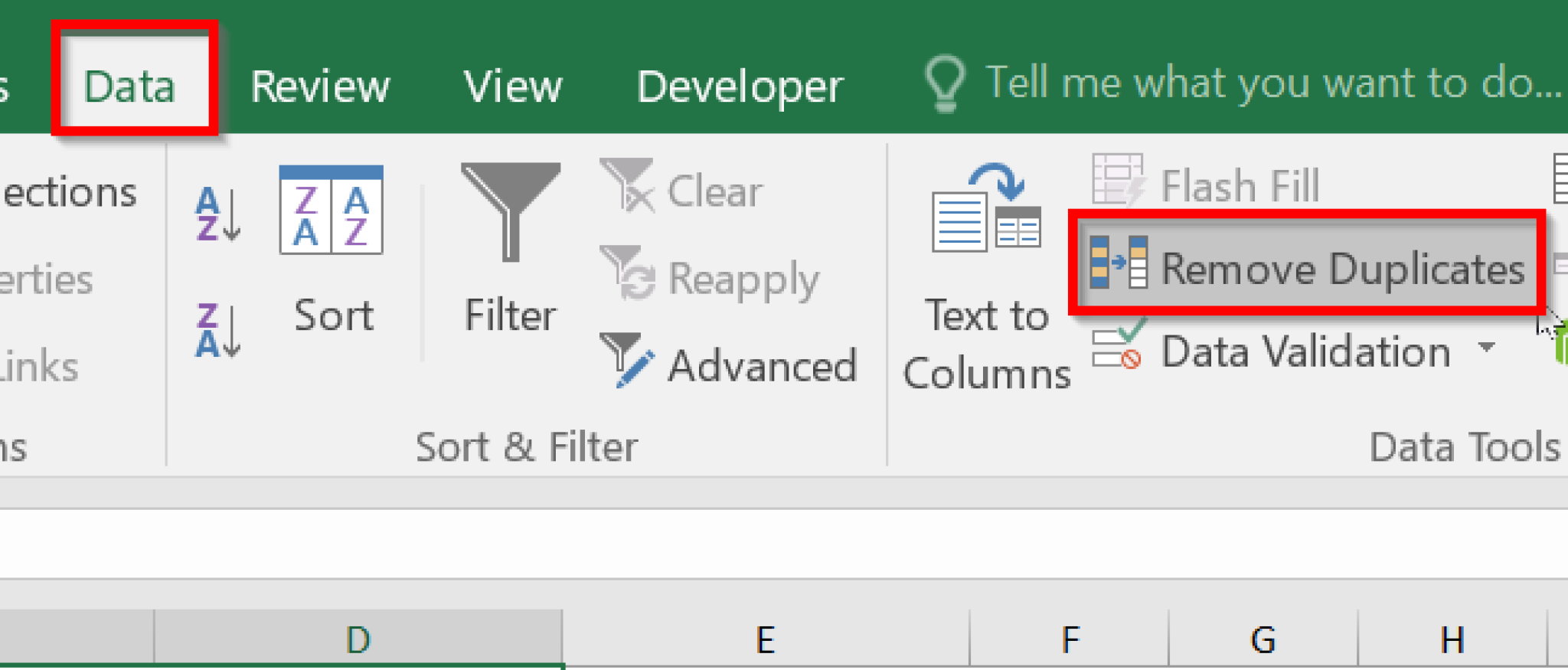
First, let's talk about how Excel identifies duplicates. It looks at the values in the cells and compares them. But here's the catch: by default, it only checks the active column. So, if you have duplicate entries across multiple columns, you need to tell Excel which columns to consider. You do this by selecting the range of cells you want to check, then heading to the "Data" tab and clicking "Remove Duplicates." A pop-up will appear, showing you the columns Excel will check. Make sure to select all the relevant columns, and voila! You're on your way to a cleaner sheet.
Setting it Up: A Step-by-Step Guide
Now, let's get into the nitty-gritty. After selecting your range, click "Remove Duplicates," and that pop-up will appear. Here, you can choose which columns to check. But be careful! If you have multiple columns with similar data, Excel might remove entries you want to keep. For example, if you have a contact list with names and email addresses, and someone has the same name but a different email, Excel might see it as a duplicate and remove one entry. To avoid this, you can use a formula like =IF(ISERROR(MATCH(B2,$B$2:$B$100,0)),"","Duplicate") in a helper column. This formula checks if the email address in column B is a duplicate within the range B2 to B100. If it is, it returns "Duplicate"; otherwise, it leaves the cell blank. This way, you can easily identify and keep the entries you need.
Another tip: before removing duplicates, consider using conditional formatting to highlight potential duplicates. This way, you can visually inspect the data and make sure you're not losing important entries. Excel's "Conditional Formatting" feature lets you format cells based on their values, so you can quickly spot and address any issues.
Keeping Your Data Clean
Maintaining a tidy spreadsheet is crucial, and remove duplicates Excel is just one tool in your belt. Regularly review and clean your data to avoid messy formatting and broken cells. Use Excel's built-in tools like SUMIFS for quick calculations and XLOOKUP for finding specific values. These formulas, along with drop-down lists and other features, can keep your sheet organized and efficient.
In a nutshell, remove duplicates Excel is a powerful feature, but it's just one part of the Excel toolkit. With a bit of practice and these tips, you'll be a pro at managing your data and keeping your spreadsheets shipshape. So, next time you open that massive contact list, remember these tricks and tackle those duplicates like a boss!
Related: How to apply the excel multiply formula for totals?
The excel multiply formula is the basic way to multiply numbers in Excel. This post shows how to use it for single cells, ranges, and simple constants.
You can apply it to multiply a column by a constant or combine it with IF for conditional calculations. If your workbook uses different versions, the syntax stays the same, though some newer functions may be available. Try the shortcut Ctrl+Shift+U to see the formula in action.
Multiply Cells, Ranges, and Constants with the excel multiply formula (asterisk operator usage)
The excel multiply formula lets you multiply a single cell, a range, or a constant using the asterisk () operator. It works the same in all Excel versions and updates instantly after pressing Enter.
To multiply a column, type the formula in the top cell and drag the fill handle down. For large ranges, a dynamic array formula can avoid manual dragging.
Combine the formula with IF for conditional multiplication, e.g., =IF(A2>10, A22, A21). In older Excel, press Ctrl+Shift+U to view the formula in the formula bar.
Requirements Before Using the excel multiply formula (apply to column)
Before you start, ensure your Excel version supports the features you need. Excel for Microsoft 365 and Excel 2019 include the full set of array functions.
All cells should contain numeric values; text will cause a #VALUE! error. If a cell might be blank, wrap the multiplication in IF to provide a default value.
Basic multiplication needs no special subscription. For newer functions like MUL, a Microsoft 365 subscription is required; check workbook trust settings if security prompts appear.
Step-by-Step Guide to Multiply a Column by a Constant
Follow these steps to multiply a column by a constant using the basic formula. The method works across Excel for Windows, Mac, and the web with minor UI differences.
- Select the column you want to multiply by clicking the column header.
- In the first cell of the column, type the constant followed by an asterisk and then the first cell reference, such as =5A2.
- Press Enter to calculate the result, then click the fill handle and drag down to copy the formula.
- For a dynamic array, use =MUL(A2:A100, 3) in Microsoft 365 or enter the array formula with Ctrl+Shift+U in older Excel.
You can also combine the excel multiply formula with IF for conditional results, e.g., =IF(A2>10, A22, A21). Ensure each part returns a number to avoid #VALUE! errors.
In older Excel, press Ctrl+Shift+U after typing the array formula to enclose it in braces. This tells Excel to treat the formula as an array operation.
Common Reasons the excel multiply formula Returns #VALUE! (zero value handling)
The #VALUE! error often appears when Excel cannot perform the multiplication because of incompatible data types. Checking the cells involved is the first step to resolve the issue. A quick way to test is to use ISNUMBER on each operand; if it returns FALSE, the cell likely contains text.
Another common cause is referencing a blank cell without a default value. Blank cells are treated as zero, which can be acceptable, but sometimes you want a specific result instead. Wrapping the multiplication in IF with a condition such as =IF(A2="",0,A2B2) avoids unexpected zeros.
- A cell contains text instead of a number.
- The formula references a blank cell, resulting in zero.
- An array formula was entered without using Ctrl+Shift+U in older Excel.
- Circular reference prevents calculation.
- Using a range that includes a header label that is text.
If the error persists after checking the cells, try saving the workbook and reopening Excel to clear any cached formula issues.
To fix the issue, convert text to numbers using Data > Text to Columns or by adding 0 to the cell, and ensure array formulas are entered with the proper shortcut. After correction, re-enter the formula and verify the result updates correctly.
Use a Dynamic Array Formula to Multiply Entire Ranges (dynamic array formula)
When you need to multiply a whole range without dragging, a dynamic array formula provides a cleaner solution. In Microsoft 365, you can use =MUL(A2:A100, 3) to multiply each element of the range by 3 and spill the results automatically. This approach eliminates the need to copy the formula manually and reduces the chance of misalignment.
If you prefer a formula that automatically expands, consider using the newer excel multiply formula with array handling, such as =MUL(A2:A100, 3). Make sure your Excel version supports the MUL function; otherwise, use the traditional =A2:A1003 array formula entered with Ctrl+Shift+U. Both methods produce the same result but differ in syntax and availability.
Another quick method is to use Paste Special to multiply a selection of cells by a constant without writing a formula. Copy the constant to the clipboard, select the range, right-click and choose Paste Special > Multiply, then OK. This technique is useful for one‑off calculations and avoids formula errors entirely.
Menus can look a bit different depending on your Excel version, but the core steps stay the same. If you’d like more Office tips, feel free to explore the other how‑to articles.
Next time you need to multiply a column, bookmark this page so you can get back to it quickly.
Related: how to move excel columns easy step by step guide
How to move Excel columns can save you a lot of time when rearranging data. Imagine you’ve got a sheet with sales data, but the "Region" column is stuck between "Product" and "Quantity," making it hard to analyze trends. Instead of copying and pasting everything, you can simply drag the column header to its new spot. It’s faster and keeps your formulas intact.
Moving columns isn’t just about aesthetics—it’s about making your data easier to work with. Whether you’re prepping a report or cleaning up a tracker, knowing how to move Excel columns ensures your sheet stays organized. Plus, it’s a skill that pairs well with other Excel tricks, like using tables or conditional formatting, to keep everything tidy.
Rearrange columns for better analysis
If you’re working with a dataset that’s out of order, moving columns is a quick fix. Analysts and project managers benefit most here, especially when dealing with logs or trackers. For example, if you’ve got a sheet tracking tasks with columns like "Priority," "Due Date," and "Status," you might want "Status" front and center for a quick glance.
Set up your sheet with clear headers in row 1 and data starting in row 2. Keep related columns together—like grouping all date fields or all numerical values. This makes it easier to apply filters or sort later. If you’re using a table (Ctrl+T), moving columns within it updates any related formulas automatically.
Here’s a sample task tracker:
| Task ID | Priority | Due Date | Status | Hours Spent |
|---|---|---|---|---|
| 001 | High | 2023-10-15 | Completed | 8 |
| 002 | Medium | 2023-10-20 | In Progress | 4 |
| 003 | Low | 2023-10-25 | Pending | 0 |
To count completed tasks, use =COUNTIFS(Status, "Completed"). This formula returns 1 in this case, since only one task is marked as done.
A common mistake here is merging cells for headers, which breaks the table structure. Always keep headers in a single row and use Center Across Selection from the Alignment tab instead.
Drag and drop with formulas intact
Moving columns with formulas requires a bit of care. If you’ve got a column calculating totals, like =B2C2 for "Total Cost," dragging the column won’t break the formula—Excel updates references automatically. This works best when your sheet uses relative references.
Start by setting up a simple invoice tracker with columns like "Item," "Price," and "Quantity." Add a "Total" column with the formula above. If you move the "Quantity" column, the formula adjusts to =D2E2 if it’s now in column D.
| Item | Price | Quantity | Total |
|---|---|---|---|
| Widget | 10 | 5 | =B2C2 |
| Gadget | 20 | 3 | =B3C3 |
To avoid errors, use =IFERROR(B2*C2, "N/A") in the Total column. This catches any division by zero or missing values, returning "N/A" instead of an error.
One mistake to avoid is hard-coding values. If you type "5" directly into a cell instead of referencing another cell, moving columns won’t update it. Always use cell references for dynamic data.
Use tables for smarter column management
Converting your data range into a table (Ctrl+T) makes moving columns even smoother. Tables automatically adjust formulas and formatting, so you don’t have to worry about breaking anything.
Tables are ideal for logs or checklists where data grows over time. For instance, a project log with columns like "Date," "Task," and "Notes" can be rearranged without messing up filters or totals.
Here’s a sample project log table:
| Date | Task | Notes | Hours |
|---|---|---|---|
| 2023-10-01 | Client Meeting | Follow-up needed | 2 |
| 2023-10-02 | Draft Proposal | Waiting on feedback | 4 |
To sum hours, use =SUM(Table1[Hours]). If you move the "Hours" column, the formula still works because tables use structured references.
A common pitfall is forgetting to expand the table when adding new columns. Always click the table, go to Table Design > Resize Table, and update the range to include new data.
Fix broken references after moving
Even with careful planning, moving columns can sometimes break formulas. If you’ve got a VLOOKUP or XLOOKUP referencing a column you moved, you’ll need to update the formula manually.
For example, if your lookup formula references column C but you moved it to column E, change =XLOOKUP(A2, C:C, D:D) to =XLOOKUP(A2, E:E, F:F).
| ID | Name | Department | Manager |
|---|---|---|---|
| 1 | John | Sales | =XLOOKUP(C2, E:E, F:F) |
| 2 | Jane | Marketing | =XLOOKUP(C3, E:E, F:F) |
To prevent this, use named ranges or tables. Go to Formulas > Define Name, select the range, and give it a name like "Departments." Then use =XLOOKUP(A2, Departments, Managers)—this stays intact even if columns move.
One mistake is not checking for numbers stored as text. If a column with numerical data is formatted as text, formulas might not work after moving. Use Data > Text to Columns to convert it back to numbers.
Try moving a column in your own sheet and adding a conditional formatting rule to highlight values above a certain threshold. It’s a quick way to see how changes affect your data.