

Excel Multiply Formula A4 Overview
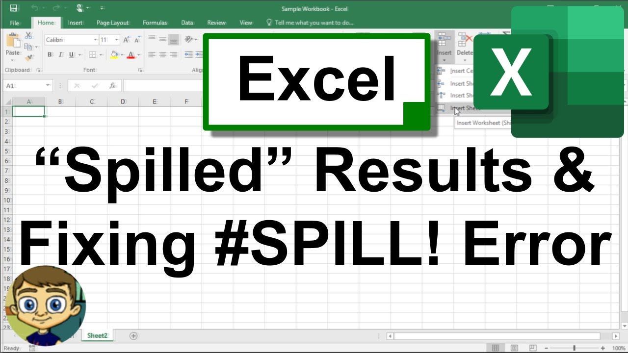
Excel spill error happens when a formula returns multiple values, but the cells below are already in use. It’s that frustrating #SPILL! message that stops your sheet cold. This usually pops up with dynamic array functions like FILTER or SORT, which can spill results into adjacent cells. If those cells are occupied, Excel throws the flag. It’s a modern problem since dynamic arrays rolled out, but the fix is straightforward once you know where to look.
Most people run into this when they’re trying to clean up a dataset or pull specific rows. For example, if you’re filtering a sales log for certain products, the FILTER function might return 20 rows, but if the 5 cells below your output are filled, you’re stuck. The error isn’t about the formula itself—it’s about the real estate on your sheet. Clear the way, and the spill works fine.
Dynamic Arrays and Why They Spill
Dynamic array functions like FILTER, UNIQUE, and SORT are a game-changer for handling lists. They automatically resize results without array formulas or manual ranges. For instance, =FILTER(A2:C100, B2:B100="Active") grabs all rows where column B says “Active.” The catch? If the output area isn’t free, you get an excel spill error. These functions don’t stop at one cell—they expand vertically or horizontally, depending on the data.
Set up your sheet with a clear output zone. I’d skip merged cells here, as they’re a recipe for spills. Use a table (Ctrl+T) for your source data, and dedicate a separate column or area for results. For example, if filtering a customer list, place the formula in cell E2 and let it spill down column E. Keep rows below empty until you’re sure how many results will appear.
| Name | Status | Date |
|---|---|---|
| John Doe | Active | 2023-01-15 |
| Jane Smith | Inactive | 2023-02-10 |
| Sam Lee | Active | 2023-03-05 |
Formula: =FILTER(A2:C4, B2:B4="Active")
This returns the first and third rows in the next column, but if cells below are filled, it triggers an excel spill error. The fix? Clear cells E2:E4 before applying the formula.
A common mistake is hard-coding values near the output area. For example, if cell E3 contains a note like “Active Customers,” the spill stops there. Delete or move static text to another column, then reapply the formula.
Troubleshooting Spills in Large Datasets
When working with hundreds of rows, an excel spill error can hide in plain sight. Maybe you filtered a dataset but forgot about hidden totals at the bottom. Or, you copied a template that had placeholder text in the spill zone. The error doesn’t care if the conflicting cell is visible—it just knows the space is taken.
For large datasets, freeze panes (View > Freeze Panes) to keep headers visible while checking the output area. Use COUNTIFS to confirm how many rows your formula should return, then compare that to the available space. For example, =COUNTIFS(B2:B100, "Active") tells you how many “Active” rows exist, so you know if your spill zone is big enough.
| Product | Sales | Region |
|------------||-----------|------------|
| Widget A | 150 | East |
| Widget B | 200 | West |
| Widget A | 180 | East |
Formula: =SORT(UNIQUE(C2:C4))
This returns unique regions in sorted order, but if cells below contain a footer, the spill fails. Use conditional formatting (Home > Conditional Formatting > Highlight Cells Rules > Blank) to spot filled cells quickly.
Another mistake is using merged cells in the output area. Excel can’t spill into a merged range, so unmerge them first (Home > Alignment > Merge & Center > Unmerge Cells).
Preventing Spills with Data Validation
Data validation isn’t just for dropdowns—it can stop spills before they start. If you know your output will never exceed 50 rows, set a validation rule to block input below that range. Go to Data > Data Validation > Settings, choose “Whole number” and set the criteria to “between” 1 and 50. This won’t stop the excel spill error, but it reminds users to clear the area first.
For a checklist or tracker, use IF and ISERROR to flag potential spills. For example, =IF(ISERROR(FILTER(A2:A10, A2:A10<>"")), "Clear cells below", "Ready") checks if the spill zone is free. Place this in a status cell to alert users.
| Task | Due Date | Status |
|---|---|---|
| Report | 2023-10-01 | Pending |
| Meeting | 2023-10-05 | Completed |
Formula: =FILTER(A2:C3, B2:B3<TODAY())
This filters overdue tasks, but if the output area contains a summary row, it fails. Add data validation to the summary row to prevent accidental input.
A common oversight is applying validation to the wrong range. Always select the exact cells below your formula, not the entire column.
Combining Spills with Pivot Tables
Pivot tables don’t cause excel spill errors, but they can work around them. If a spill zone is too crowded, summarize the data in a pivot instead. Select your table, go to Insert > PivotTable, and drag fields to Rows and Values. For example, pivot the sales data by region without worrying about spills.
For a hybrid approach, use UNIQUE to extract distinct values, then reference them in a pivot. Formula: =UNIQUE(C2:C100). This spills unique regions into a column, which you can then use as a source for your pivot table.
| Region | Sales |
|---|---|
| East | 330 |
| West | 200 |
The pivot table summarizes without needing a spill zone, but if you still want dynamic arrays, link the UNIQUE output to a separate tab.
One mistake is mixing pivot data with spill ranges. Keep pivots on their own sheet or tab to avoid conflicts.
Try setting up a small tracker with FILTER and intentionally trigger an excel spill error. Then, clear the output area and watch the formula work. It’s a quick way to see how spills behave in your own file.
Related: Excel remove blank rows using filter and delete
You just pasted a big list into Excel and now half the rows are empty, so you need to excel remove blank rows quickly. You can start by using Excel’s filter to hide blank rows, which is the first step in excel remove blank rows.
First, select your data range and turn on the filter from the Data tab; then click the drop‑down arrow on any column header and uncheck the blank option to hide them. After you filter, you can delete the hidden rows, or copy the visible rows to a new sheet to finish the delete empty rows excel cleanup.
How to excel remove blank rows and keep data tidy
When you paste a large list into Excel, many rows can appear empty because of trailing spaces or hidden cells. Turning on the filter lets you hide those rows instantly. Using filter blank rows gives a quick visual check of which rows are truly blank.
After filtering, you have two options: delete the hidden rows or copy the visible rows to a new sheet. Both give a dataset without empty lines, which makes sorting and charting smoother. The delete empty rows excel command can be added to a toolbar for fast access.
If you prefer a one‑click delete, select the filtered rows, right‑click and choose Delete Rows, or use the Delete key after selecting the entire range.
If you work with a table, convert the range first; tables update automatically and keep blank rows out of future imports.
What you need before you start (Excel version and account)
The filter method works in Excel 2016 and newer, including Excel for Microsoft 365 and Excel 2019. If you are on an older version, you can still hide rows manually, but the built‑in filter arrow will not appear. Make sure the file is a workbook (.xlsx) and not protected, because protection blocks row deletion.
Before deleting, turn on the filter from the Data tab. In a Microsoft 365 corporate account, an admin may have disabled the filter. Ask the administrator to enable it or copy the data to a personal workbook where you have control.
If the filter still shows blank rows, check for hidden columns that contain data; unhide them before filtering to ensure all empty rows are detected.
For very large sheets, consider splitting the data into multiple workbooks; each smaller file loads faster and reduces filter lag.
Step‑by‑step method to delete empty rows
Use the filter to hide blank rows, then delete them in Excel quickly.
- Select any cell in your data range and click Filter on the Data tab to show dropdown arrows.
- Click a column dropdown, scroll to the bottom, and uncheck the blank option; repeat for any other column you want to filter.
- Excel will hide rows with no data in the selected columns. Verify that only the rows you need remain visible.
- To delete the hidden rows, select the row numbers, right‑click and choose Delete Rows, or press Delete after selecting the entire row range.
- If you prefer not to delete, copy the visible rows to a new sheet by selecting, copying, and pasting them into a blank workbook for backup.
Save the workbook to keep the changes. Your data now contains only rows with actual content.
Why it may not work and what to check
If blank rows still appear after filtering, check these common causes in Excel quickly before trying other methods to save time.
- Make sure the column you filter actually contains data; an empty column will not show the blank option.
- Verify the filter dropdown arrow is visible; a missing arrow means the filter is disabled for that sheet.
- If the workbook is protected, you cannot delete rows; unprotect it via the Review tab before proceeding.
- Trailing spaces can hide data from the filter; run trim whitespace excel on the column to remove them.
- Hidden columns may contain data; unhide them before filtering so the blank rows become visible and can be removed.
After fixing the issue, run the filter again to confirm no blank rows remain, then save the file.
If you still see blank rows, try sorting the column; sorted order often reveals hidden empty cells that the filter missed.
Safer alternative and how to prevent blank rows next time
A more durable way to excel remove blank rows is to convert your range into an Excel table. Tables automatically expand when you add data and have a built‑in filter that shows only non‑blank rows, so you never have to repeat the cleanup process.
To avoid blank rows in the first place, clean the source data before pasting: use Find & Select > Replace to remove extra spaces, then paste into the sheet. After pasting, run the Remove Blank Cells command from the Home tab to purge any lingering empty rows. Keeping a table and refreshing its data range also prevents stray blank lines from reappearing.
Flag blanks in a helper column, filter, and delete rows in one step.
Menus can look a bit different depending on your Excel version, so if something doesn’t match the screenshots just hunt for the similar command. You can also browse other quick Office tips for more handy tricks.
If this helped, feel free to bookmark the page for the next time you need to clean up blank rows.
Related: How to apply the excel multiply formula for totals?
The excel multiply formula is the basic way to multiply numbers in Excel. This post shows how to use it for single cells, ranges, and simple constants.
You can apply it to multiply a column by a constant or combine it with IF for conditional calculations. If your workbook uses different versions, the syntax stays the same, though some newer functions may be available. Try the shortcut Ctrl+Shift+U to see the formula in action.
Multiply Cells, Ranges, and Constants with the excel multiply formula (asterisk operator usage)
The excel multiply formula lets you multiply a single cell, a range, or a constant using the asterisk () operator. It works the same in all Excel versions and updates instantly after pressing Enter.
To multiply a column, type the formula in the top cell and drag the fill handle down. For large ranges, a dynamic array formula can avoid manual dragging.
Combine the formula with IF for conditional multiplication, e.g., =IF(A2>10, A22, A21). In older Excel, press Ctrl+Shift+U to view the formula in the formula bar.
Requirements Before Using the excel multiply formula (apply to column)
Before you start, ensure your Excel version supports the features you need. Excel for Microsoft 365 and Excel 2019 include the full set of array functions.
All cells should contain numeric values; text will cause a #VALUE! error. If a cell might be blank, wrap the multiplication in IF to provide a default value.
Basic multiplication needs no special subscription. For newer functions like MUL, a Microsoft 365 subscription is required; check workbook trust settings if security prompts appear.
Step-by-Step Guide to Multiply a Column by a Constant
Follow these steps to multiply a column by a constant using the basic formula. The method works across Excel for Windows, Mac, and the web with minor UI differences.
- Select the column you want to multiply by clicking the column header.
- In the first cell of the column, type the constant followed by an asterisk and then the first cell reference, such as =5A2.
- Press Enter to calculate the result, then click the fill handle and drag down to copy the formula.
- For a dynamic array, use =MUL(A2:A100, 3) in Microsoft 365 or enter the array formula with Ctrl+Shift+U in older Excel.
You can also combine the excel multiply formula with IF for conditional results, e.g., =IF(A2>10, A22, A21). Ensure each part returns a number to avoid #VALUE! errors.
In older Excel, press Ctrl+Shift+U after typing the array formula to enclose it in braces. This tells Excel to treat the formula as an array operation.
Common Reasons the excel multiply formula Returns #VALUE! (zero value handling)
The #VALUE! error often appears when Excel cannot perform the multiplication because of incompatible data types. Checking the cells involved is the first step to resolve the issue. A quick way to test is to use ISNUMBER on each operand; if it returns FALSE, the cell likely contains text.
Another common cause is referencing a blank cell without a default value. Blank cells are treated as zero, which can be acceptable, but sometimes you want a specific result instead. Wrapping the multiplication in IF with a condition such as =IF(A2="",0,A2B2) avoids unexpected zeros.
- A cell contains text instead of a number.
- The formula references a blank cell, resulting in zero.
- An array formula was entered without using Ctrl+Shift+U in older Excel.
- Circular reference prevents calculation.
- Using a range that includes a header label that is text.
If the error persists after checking the cells, try saving the workbook and reopening Excel to clear any cached formula issues.
To fix the issue, convert text to numbers using Data > Text to Columns or by adding 0 to the cell, and ensure array formulas are entered with the proper shortcut. After correction, re-enter the formula and verify the result updates correctly.
Use a Dynamic Array Formula to Multiply Entire Ranges (dynamic array formula)
When you need to multiply a whole range without dragging, a dynamic array formula provides a cleaner solution. In Microsoft 365, you can use =MUL(A2:A100, 3) to multiply each element of the range by 3 and spill the results automatically. This approach eliminates the need to copy the formula manually and reduces the chance of misalignment.
If you prefer a formula that automatically expands, consider using the newer excel multiply formula with array handling, such as =MUL(A2:A100, 3). Make sure your Excel version supports the MUL function; otherwise, use the traditional =A2:A1003 array formula entered with Ctrl+Shift+U. Both methods produce the same result but differ in syntax and availability.
Another quick method is to use Paste Special to multiply a selection of cells by a constant without writing a formula. Copy the constant to the clipboard, select the range, right-click and choose Paste Special > Multiply, then OK. This technique is useful for one‑off calculations and avoids formula errors entirely.
Menus can look a bit different depending on your Excel version, but the core steps stay the same. If you’d like more Office tips, feel free to explore the other how‑to articles.
Next time you need to multiply a column, bookmark this page so you can get back to it quickly.