

Excel Sum Formula Free Printable Overview
How to move Excel columns can save you a lot of time when rearranging data. Imagine you’ve got a sheet with sales data, but the "Region" column is stuck between "Product" and "Quantity," making it hard to analyze trends. Instead of copying and pasting everything, you can simply drag the column header to its new spot. It’s faster and keeps your formulas intact.
Moving columns isn’t just about aesthetics—it’s about making your data easier to work with. Whether you’re prepping a report or cleaning up a tracker, knowing how to move Excel columns ensures your sheet stays organized. Plus, it’s a skill that pairs well with other Excel tricks, like using tables or conditional formatting, to keep everything tidy.
Rearrange columns for better analysis
If you’re working with a dataset that’s out of order, moving columns is a quick fix. Analysts and project managers benefit most here, especially when dealing with logs or trackers. For example, if you’ve got a sheet tracking tasks with columns like "Priority," "Due Date," and "Status," you might want "Status" front and center for a quick glance.
Set up your sheet with clear headers in row 1 and data starting in row 2. Keep related columns together—like grouping all date fields or all numerical values. This makes it easier to apply filters or sort later. If you’re using a table (Ctrl+T), moving columns within it updates any related formulas automatically.
Here’s a sample task tracker:
| Task ID | Priority | Due Date | Status | Hours Spent |
|---|---|---|---|---|
| 001 | High | 2023-10-15 | Completed | 8 |
| 002 | Medium | 2023-10-20 | In Progress | 4 |
| 003 | Low | 2023-10-25 | Pending | 0 |
To count completed tasks, use =COUNTIFS(Status, "Completed"). This formula returns 1 in this case, since only one task is marked as done.
A common mistake here is merging cells for headers, which breaks the table structure. Always keep headers in a single row and use Center Across Selection from the Alignment tab instead.
Drag and drop with formulas intact
Moving columns with formulas requires a bit of care. If you’ve got a column calculating totals, like =B2C2 for "Total Cost," dragging the column won’t break the formula—Excel updates references automatically. This works best when your sheet uses relative references.
Start by setting up a simple invoice tracker with columns like "Item," "Price," and "Quantity." Add a "Total" column with the formula above. If you move the "Quantity" column, the formula adjusts to =D2E2 if it’s now in column D.
| Item | Price | Quantity | Total |
|---|---|---|---|
| Widget | 10 | 5 | =B2C2 |
| Gadget | 20 | 3 | =B3C3 |
To avoid errors, use =IFERROR(B2*C2, "N/A") in the Total column. This catches any division by zero or missing values, returning "N/A" instead of an error.
One mistake to avoid is hard-coding values. If you type "5" directly into a cell instead of referencing another cell, moving columns won’t update it. Always use cell references for dynamic data.
Use tables for smarter column management
Converting your data range into a table (Ctrl+T) makes moving columns even smoother. Tables automatically adjust formulas and formatting, so you don’t have to worry about breaking anything.
Tables are ideal for logs or checklists where data grows over time. For instance, a project log with columns like "Date," "Task," and "Notes" can be rearranged without messing up filters or totals.
Here’s a sample project log table:
| Date | Task | Notes | Hours |
|---|---|---|---|
| 2023-10-01 | Client Meeting | Follow-up needed | 2 |
| 2023-10-02 | Draft Proposal | Waiting on feedback | 4 |
To sum hours, use =SUM(Table1[Hours]). If you move the "Hours" column, the formula still works because tables use structured references.
A common pitfall is forgetting to expand the table when adding new columns. Always click the table, go to Table Design > Resize Table, and update the range to include new data.
Fix broken references after moving
Even with careful planning, moving columns can sometimes break formulas. If you’ve got a VLOOKUP or XLOOKUP referencing a column you moved, you’ll need to update the formula manually.
For example, if your lookup formula references column C but you moved it to column E, change =XLOOKUP(A2, C:C, D:D) to =XLOOKUP(A2, E:E, F:F).
| ID | Name | Department | Manager |
|---|---|---|---|
| 1 | John | Sales | =XLOOKUP(C2, E:E, F:F) |
| 2 | Jane | Marketing | =XLOOKUP(C3, E:E, F:F) |
To prevent this, use named ranges or tables. Go to Formulas > Define Name, select the range, and give it a name like "Departments." Then use =XLOOKUP(A2, Departments, Managers)—this stays intact even if columns move.
One mistake is not checking for numbers stored as text. If a column with numerical data is formatted as text, formulas might not work after moving. Use Data > Text to Columns to convert it back to numbers.
Try moving a column in your own sheet and adding a conditional formatting rule to highlight values above a certain threshold. It’s a quick way to see how changes affect your data.
Related: excel spill error Easy guide to fix and prevent issues
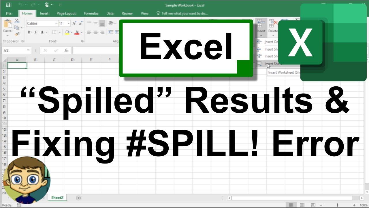
Excel spill error happens when a formula returns multiple values, but the cells below are already in use. It’s that frustrating #SPILL! message that stops your sheet cold. This usually pops up with dynamic array functions like FILTER or SORT, which can spill results into adjacent cells. If those cells are occupied, Excel throws the flag. It’s a modern problem since dynamic arrays rolled out, but the fix is straightforward once you know where to look.
Most people run into this when they’re trying to clean up a dataset or pull specific rows. For example, if you’re filtering a sales log for certain products, the FILTER function might return 20 rows, but if the 5 cells below your output are filled, you’re stuck. The error isn’t about the formula itself—it’s about the real estate on your sheet. Clear the way, and the spill works fine.
Dynamic Arrays and Why They Spill
Dynamic array functions like FILTER, UNIQUE, and SORT are a game-changer for handling lists. They automatically resize results without array formulas or manual ranges. For instance, =FILTER(A2:C100, B2:B100="Active") grabs all rows where column B says “Active.” The catch? If the output area isn’t free, you get an excel spill error. These functions don’t stop at one cell—they expand vertically or horizontally, depending on the data.
Set up your sheet with a clear output zone. I’d skip merged cells here, as they’re a recipe for spills. Use a table (Ctrl+T) for your source data, and dedicate a separate column or area for results. For example, if filtering a customer list, place the formula in cell E2 and let it spill down column E. Keep rows below empty until you’re sure how many results will appear.
| Name | Status | Date |
|---|---|---|
| John Doe | Active | 2023-01-15 |
| Jane Smith | Inactive | 2023-02-10 |
| Sam Lee | Active | 2023-03-05 |
Formula: =FILTER(A2:C4, B2:B4="Active")
This returns the first and third rows in the next column, but if cells below are filled, it triggers an excel spill error. The fix? Clear cells E2:E4 before applying the formula.
A common mistake is hard-coding values near the output area. For example, if cell E3 contains a note like “Active Customers,” the spill stops there. Delete or move static text to another column, then reapply the formula.
Troubleshooting Spills in Large Datasets
When working with hundreds of rows, an excel spill error can hide in plain sight. Maybe you filtered a dataset but forgot about hidden totals at the bottom. Or, you copied a template that had placeholder text in the spill zone. The error doesn’t care if the conflicting cell is visible—it just knows the space is taken.
For large datasets, freeze panes (View > Freeze Panes) to keep headers visible while checking the output area. Use COUNTIFS to confirm how many rows your formula should return, then compare that to the available space. For example, =COUNTIFS(B2:B100, "Active") tells you how many “Active” rows exist, so you know if your spill zone is big enough.
| Product | Sales | Region |
|------------||-----------|------------|
| Widget A | 150 | East |
| Widget B | 200 | West |
| Widget A | 180 | East |
Formula: =SORT(UNIQUE(C2:C4))
This returns unique regions in sorted order, but if cells below contain a footer, the spill fails. Use conditional formatting (Home > Conditional Formatting > Highlight Cells Rules > Blank) to spot filled cells quickly.
Another mistake is using merged cells in the output area. Excel can’t spill into a merged range, so unmerge them first (Home > Alignment > Merge & Center > Unmerge Cells).
Preventing Spills with Data Validation
Data validation isn’t just for dropdowns—it can stop spills before they start. If you know your output will never exceed 50 rows, set a validation rule to block input below that range. Go to Data > Data Validation > Settings, choose “Whole number” and set the criteria to “between” 1 and 50. This won’t stop the excel spill error, but it reminds users to clear the area first.
For a checklist or tracker, use IF and ISERROR to flag potential spills. For example, =IF(ISERROR(FILTER(A2:A10, A2:A10<>"")), "Clear cells below", "Ready") checks if the spill zone is free. Place this in a status cell to alert users.
| Task | Due Date | Status |
|---|---|---|
| Report | 2023-10-01 | Pending |
| Meeting | 2023-10-05 | Completed |
Formula: =FILTER(A2:C3, B2:B3<TODAY())
This filters overdue tasks, but if the output area contains a summary row, it fails. Add data validation to the summary row to prevent accidental input.
A common oversight is applying validation to the wrong range. Always select the exact cells below your formula, not the entire column.
Combining Spills with Pivot Tables
Pivot tables don’t cause excel spill errors, but they can work around them. If a spill zone is too crowded, summarize the data in a pivot instead. Select your table, go to Insert > PivotTable, and drag fields to Rows and Values. For example, pivot the sales data by region without worrying about spills.
For a hybrid approach, use UNIQUE to extract distinct values, then reference them in a pivot. Formula: =UNIQUE(C2:C100). This spills unique regions into a column, which you can then use as a source for your pivot table.
| Region | Sales |
|---|---|
| East | 330 |
| West | 200 |
The pivot table summarizes without needing a spill zone, but if you still want dynamic arrays, link the UNIQUE output to a separate tab.
One mistake is mixing pivot data with spill ranges. Keep pivots on their own sheet or tab to avoid conflicts.
Try setting up a small tracker with FILTER and intentionally trigger an excel spill error. Then, clear the output area and watch the formula work. It’s a quick way to see how spills behave in your own file.
Related: Create a Sankey Chart in Excel: A Simple Guide
A common misconception about sankey chart excel is that it's solely for engineers or data experts. But, in reality, anyone can benefit from understanding these visual gems!
Sankey diagrams offer a simple yet powerful way to visualize flows and processes. Whether tracking energy, materials, or any other data, they provide an at-a-glance overview, making complex information accessible. So, if you've been avoiding sankey chart excel, it's time to give it a go! You might just discover a new favorite tool.
Understanding the Flow: Sankey Chart Excel
Sankey charts are a powerful tool to visualize the flow of data, often used to show energy or material balances in a process. These charts are a great way to understand complex systems and their components. In this guide, we'll explore how to read and create Sankey charts in Excel, making data analysis a breeze!
Comparing Chart Options: Sankey vs. Other Visualizations
When it comes to data visualization, Sankey charts offer a unique perspective. Unlike bar charts or line graphs, Sankey diagrams focus on the flow and connection between categories. They are ideal for showing how one category contributes to another, making them perfect for energy flow analyses or tracking material usage.
Creating a Sankey: A Step-by-Step Guide
To create a Sankey chart in Excel, follow these simple steps:
Gather your data: Ensure you have a clear understanding of the categories and their relationships. Organize your data in a structured way, with columns representing the flow sources and targets.
Prepare your data: Clean and format your data to ensure accuracy. Convert any necessary units and ensure consistent formatting. Excel's data validation tools can help with this process.
Insert the Sankey chart: Go to the 'Insert' tab in Excel and select 'Recommended Charts'. Choose the 'All Charts' tab, and under the 'Hierarchy' section, select 'Sankey'. Excel will suggest a layout based on your data.
Customize and refine: Adjust the chart's appearance to your liking. Change colors, add labels, and format the text to enhance readability. You can also adjust the width of the flow arrows to emphasize important data points.
Interpret the results: Analyze the chart to understand the flow patterns. Look for areas where the flow is concentrated or where there are significant drops or increases. This visualization will help identify key trends and areas of interest.
Common Misreadings and Pitfalls
While Sankey charts are powerful, they can be misinterpreted if not read correctly. Here are some common mistakes to avoid:
Misinterpreting arrow width: The width of the arrows represents the flow magnitude. Wider arrows indicate a larger flow, but this can be misleading if the scale is not considered. Always check the legend or scale to understand the actual values.
Ignoring labels: Sankey charts often have labels along the arrows, providing additional context. These labels can indicate the specific category or the flow rate. Ensure you read and understand these labels to gain a comprehensive understanding.
Overlooking data ranges: Sankey charts may not always represent the full range of values. If the chart only shows a subset of data, ensure you understand the boundaries and consider the complete dataset for accurate analysis.
Key Factors Affecting Accuracy
To ensure accurate Sankey charts, consider these critical factors:
Data integrity: Ensure your data is accurate and up-to-date. Any errors or inconsistencies can lead to misleading visualizations.
Standard units: Always use consistent units throughout your data. Mixing units can result in incorrect flow representations.
Scale and range: Understand the scale and range of your data. Sankey charts may not always show the full range, so consider the boundaries and potential outliers.
Data normalization: If your data has vastly different scales, consider normalizing it to ensure an accurate representation. This step is crucial when comparing flows of varying magnitudes.
Adapting the Format: Real-World Applications
Sankey charts excel in various real-world applications. Here are some ways to adapt the format for specific needs:
Energy audits: Visualize energy flows in a building or industrial process to identify inefficiencies and optimize energy usage.
Material tracking: Track the flow of materials in a supply chain, helping to identify bottlenecks and optimize resource allocation.
Process optimization: Analyze process flows in manufacturing or chemical engineering to improve efficiency and reduce waste.
Environmental impact: Assess the environmental impact of a process by visualizing the flow of emissions or waste products.
Customer journey mapping: Map customer interactions and journeys, helping businesses understand customer behavior and improve their experience.
Hey there, I hope this guide has given you a clear understanding of sankey charts in Excel. Remember, the specifics may differ slightly based on your Excel version or the data you're working with, so always double-check your sources and adapt as needed.
Feel free to explore our other guides; we've got plenty of practical tips and tricks to help you master various tools and techniques. Happy charting!