

Excel Sum Formula Letter Size Overview
Ugh, duplicates in Excel. We've all been there, staring at a massive spreadsheet with rows and rows of data, only to realize there are multiple entries for the same thing. Remove duplicates Excel to the rescue! Let's get into how this handy feature works and why it's a lifesaver for anyone dealing with data.
So, you've got your Excel sheet open, and it's a mess of similar entries. Maybe it's a list of contacts, products, or sales data, and you need to clean it up. The "Remove Duplicates" feature is like a magic wand, but it's not as simple as clicking a button. You've got to set it up right to get the results you need.
First, let's talk about how Excel identifies duplicates. It looks at the values in the cells and compares them. But here's the catch: by default, it only checks the active column. So, if you have duplicate entries across multiple columns, you need to tell Excel which columns to consider. You do this by selecting the range of cells you want to check, then heading to the "Data" tab and clicking "Remove Duplicates." A pop-up will appear, showing you the columns Excel will check. Make sure to select all the relevant columns, and voila! You're on your way to a cleaner sheet.
Setting it Up: A Step-by-Step Guide
Now, let's get into the nitty-gritty. After selecting your range, click "Remove Duplicates," and that pop-up will appear. Here, you can choose which columns to check. But be careful! If you have multiple columns with similar data, Excel might remove entries you want to keep. For example, if you have a contact list with names and email addresses, and someone has the same name but a different email, Excel might see it as a duplicate and remove one entry. To avoid this, you can use a formula like =IF(ISERROR(MATCH(B2,$B$2:$B$100,0)),"","Duplicate") in a helper column. This formula checks if the email address in column B is a duplicate within the range B2 to B100. If it is, it returns "Duplicate"; otherwise, it leaves the cell blank. This way, you can easily identify and keep the entries you need.
Another tip: before removing duplicates, consider using conditional formatting to highlight potential duplicates. This way, you can visually inspect the data and make sure you're not losing important entries. Excel's "Conditional Formatting" feature lets you format cells based on their values, so you can quickly spot and address any issues.
Keeping Your Data Clean
Maintaining a tidy spreadsheet is crucial, and remove duplicates Excel is just one tool in your belt. Regularly review and clean your data to avoid messy formatting and broken cells. Use Excel's built-in tools like SUMIFS for quick calculations and XLOOKUP for finding specific values. These formulas, along with drop-down lists and other features, can keep your sheet organized and efficient.
In a nutshell, remove duplicates Excel is a powerful feature, but it's just one part of the Excel toolkit. With a bit of practice and these tips, you'll be a pro at managing your data and keeping your spreadsheets shipshape. So, next time you open that massive contact list, remember these tricks and tackle those duplicates like a boss!
Related: Create a Sankey Chart in Excel: A Simple Guide
A common misconception about sankey chart excel is that it's solely for engineers or data experts. But, in reality, anyone can benefit from understanding these visual gems!
Sankey diagrams offer a simple yet powerful way to visualize flows and processes. Whether tracking energy, materials, or any other data, they provide an at-a-glance overview, making complex information accessible. So, if you've been avoiding sankey chart excel, it's time to give it a go! You might just discover a new favorite tool.
Understanding the Flow: Sankey Chart Excel
Sankey charts are a powerful tool to visualize the flow of data, often used to show energy or material balances in a process. These charts are a great way to understand complex systems and their components. In this guide, we'll explore how to read and create Sankey charts in Excel, making data analysis a breeze!
Comparing Chart Options: Sankey vs. Other Visualizations
When it comes to data visualization, Sankey charts offer a unique perspective. Unlike bar charts or line graphs, Sankey diagrams focus on the flow and connection between categories. They are ideal for showing how one category contributes to another, making them perfect for energy flow analyses or tracking material usage.
Creating a Sankey: A Step-by-Step Guide
To create a Sankey chart in Excel, follow these simple steps:
Gather your data: Ensure you have a clear understanding of the categories and their relationships. Organize your data in a structured way, with columns representing the flow sources and targets.
Prepare your data: Clean and format your data to ensure accuracy. Convert any necessary units and ensure consistent formatting. Excel's data validation tools can help with this process.
Insert the Sankey chart: Go to the 'Insert' tab in Excel and select 'Recommended Charts'. Choose the 'All Charts' tab, and under the 'Hierarchy' section, select 'Sankey'. Excel will suggest a layout based on your data.
Customize and refine: Adjust the chart's appearance to your liking. Change colors, add labels, and format the text to enhance readability. You can also adjust the width of the flow arrows to emphasize important data points.
Interpret the results: Analyze the chart to understand the flow patterns. Look for areas where the flow is concentrated or where there are significant drops or increases. This visualization will help identify key trends and areas of interest.
Common Misreadings and Pitfalls
While Sankey charts are powerful, they can be misinterpreted if not read correctly. Here are some common mistakes to avoid:
Misinterpreting arrow width: The width of the arrows represents the flow magnitude. Wider arrows indicate a larger flow, but this can be misleading if the scale is not considered. Always check the legend or scale to understand the actual values.
Ignoring labels: Sankey charts often have labels along the arrows, providing additional context. These labels can indicate the specific category or the flow rate. Ensure you read and understand these labels to gain a comprehensive understanding.
Overlooking data ranges: Sankey charts may not always represent the full range of values. If the chart only shows a subset of data, ensure you understand the boundaries and consider the complete dataset for accurate analysis.
Key Factors Affecting Accuracy
To ensure accurate Sankey charts, consider these critical factors:
Data integrity: Ensure your data is accurate and up-to-date. Any errors or inconsistencies can lead to misleading visualizations.
Standard units: Always use consistent units throughout your data. Mixing units can result in incorrect flow representations.
Scale and range: Understand the scale and range of your data. Sankey charts may not always show the full range, so consider the boundaries and potential outliers.
Data normalization: If your data has vastly different scales, consider normalizing it to ensure an accurate representation. This step is crucial when comparing flows of varying magnitudes.
Adapting the Format: Real-World Applications
Sankey charts excel in various real-world applications. Here are some ways to adapt the format for specific needs:
Energy audits: Visualize energy flows in a building or industrial process to identify inefficiencies and optimize energy usage.
Material tracking: Track the flow of materials in a supply chain, helping to identify bottlenecks and optimize resource allocation.
Process optimization: Analyze process flows in manufacturing or chemical engineering to improve efficiency and reduce waste.
Environmental impact: Assess the environmental impact of a process by visualizing the flow of emissions or waste products.
Customer journey mapping: Map customer interactions and journeys, helping businesses understand customer behavior and improve their experience.
Hey there, I hope this guide has given you a clear understanding of sankey charts in Excel. Remember, the specifics may differ slightly based on your Excel version or the data you're working with, so always double-check your sources and adapt as needed.
Feel free to explore our other guides; we've got plenty of practical tips and tricks to help you master various tools and techniques. Happy charting!
Related: how to create pivot chart Easy guide for Excel users
I've been working with spreadsheets for a while now, and one of the most useful skills I've learned is how to create pivot charts. It's a game-changer for visualizing data and making sense of complex information. So, let's dive into the process and see how we can make our data pop with these dynamic charts!
Setting Up Your Data for Success
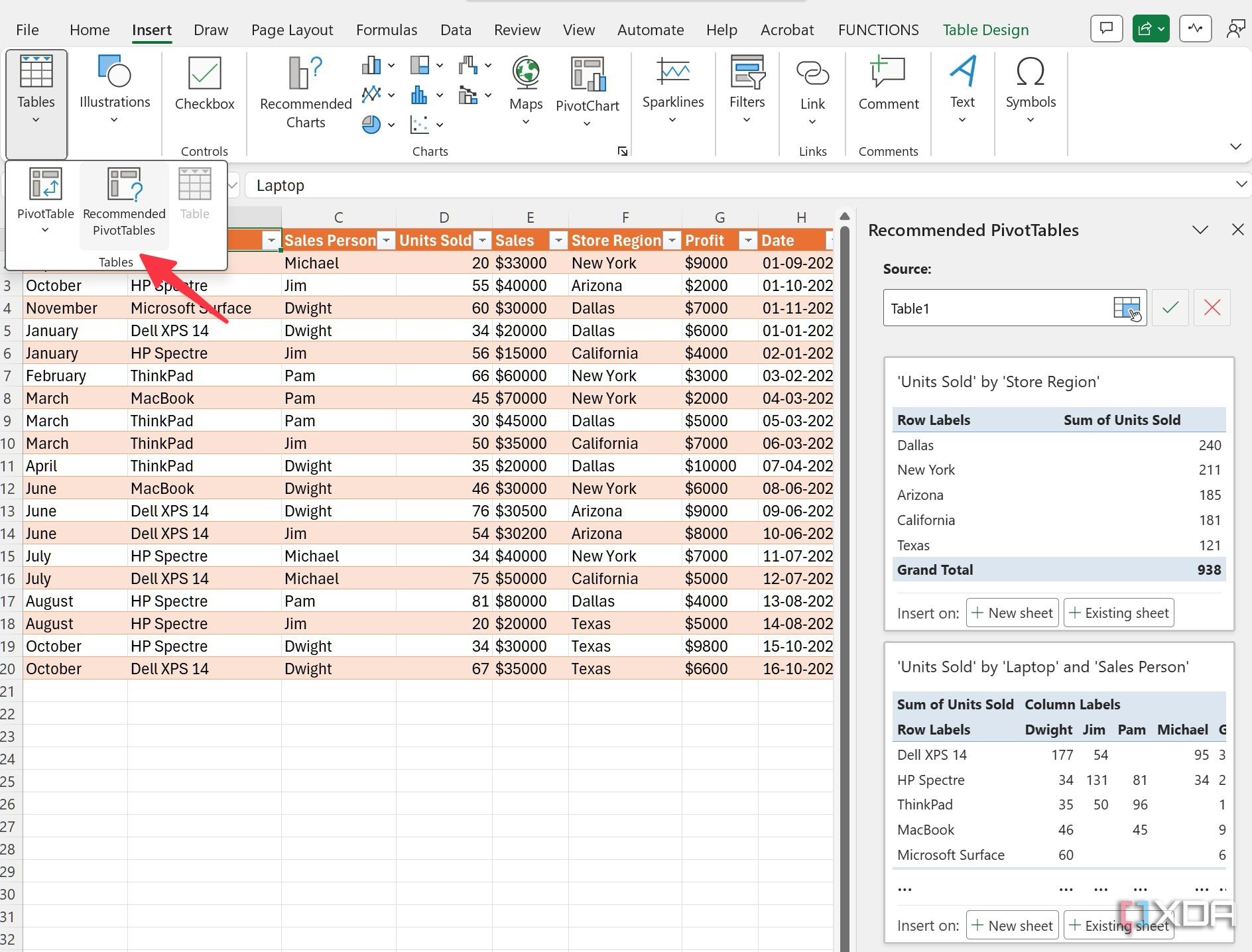
When it comes to creating pivot charts, the first step is ensuring your data is structured properly. Think of your spreadsheet as a house; the columns are the rooms, and the rows are the items within each room. So, before we start, let's tidy up our data: make sure your columns have clear, concise headers, and your rows are consistent and organized. This step is crucial because it lays the foundation for an accurate and effective pivot chart.
Now, let's talk about the tools Excel provides to make this process smoother. Excel has some fantastic built-in features to help with data manipulation and formatting. For instance, you can use the XLOOKUP formula to quickly find and retrieve specific data points, or the IF function to create conditional rules for your data. These formulas are your friends and can save you a lot of time and effort, especially when dealing with large datasets.
Building Your Pivot Chart
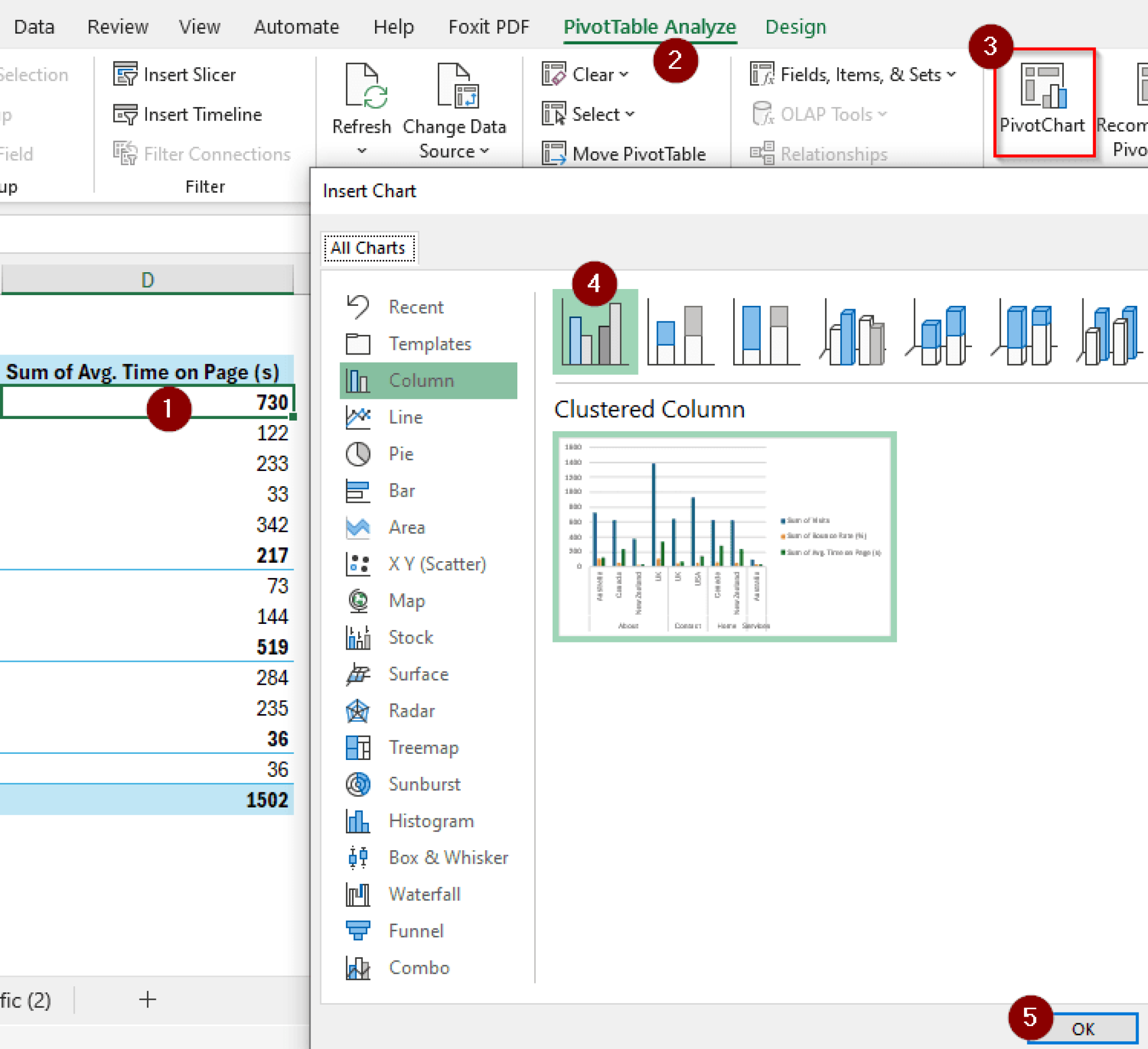
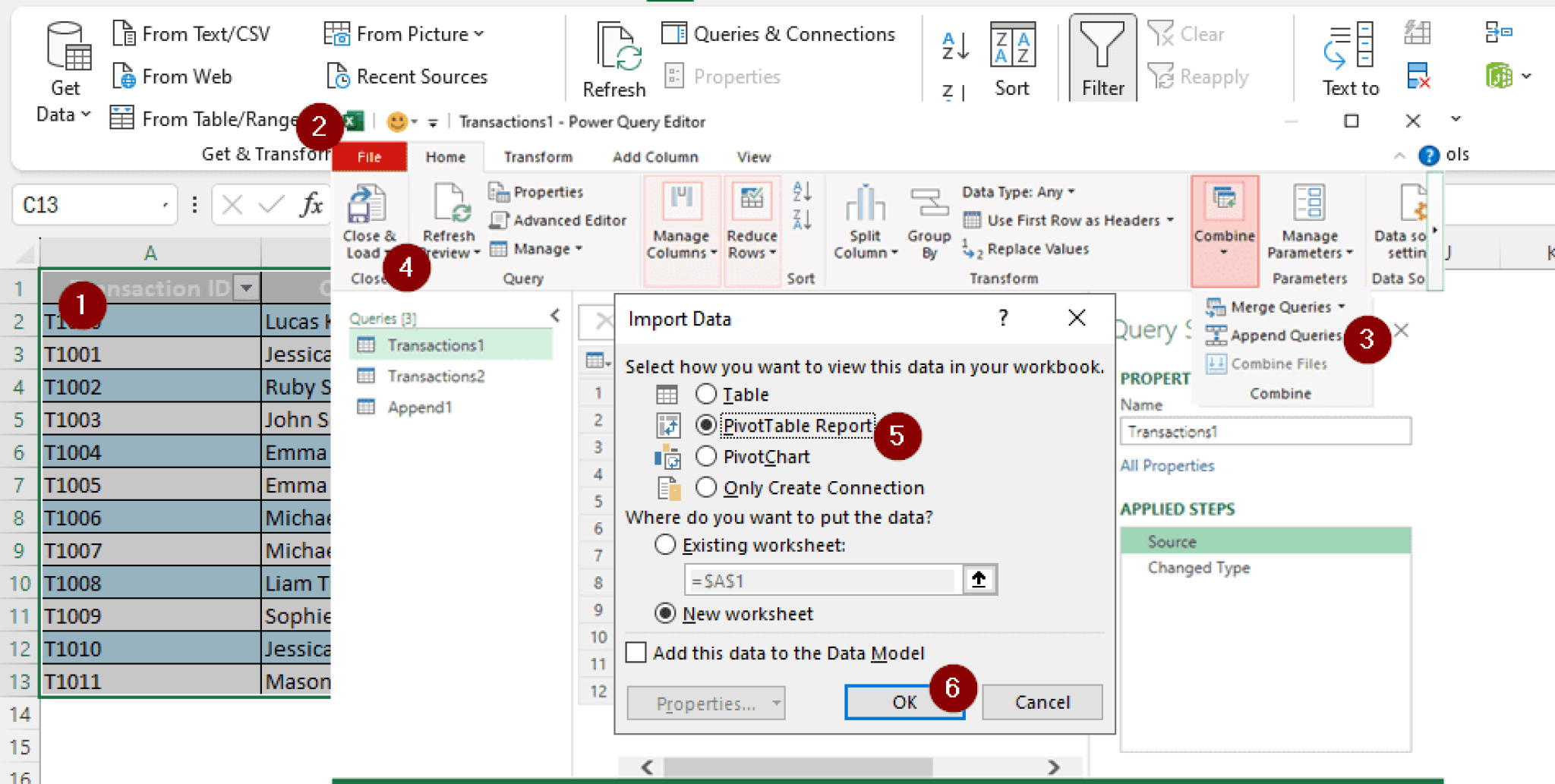
Once your data is shipshape, it's time to build your pivot chart. Excel makes this process pretty straightforward. Go to the Insert tab and select PivotChart. From here, you'll be prompted to choose the data range you want to include in your chart. Excel will then display a new window where you can customize your chart's layout.
This is where the magic happens! You can drag and drop fields to create rows, columns, and even filters for your chart. For example, if you have a dataset with sales data, you could drag the "Product" field to the Rows area, and the "Sales Amount" field to the Values area. This will create a chart that shows the sales performance of each product.
Customizing and Refining
Now that you have your basic pivot chart, it's time to add some polish. Excel offers a range of customization options to make your chart truly shine. You can change the chart type, add titles and labels, and even apply conditional formatting to highlight specific data points. For instance, you could use conditional formatting to highlight cells with sales above a certain threshold, making it easy to identify top-performing products at a glance.
Another useful feature is the ability to create drop-down lists in your pivot chart. This allows you to quickly filter your data by selecting different options from a drop-down menu. It's a great way to make your chart more interactive and user-friendly.
Final Thoughts
So, there you have it! Creating pivot charts in Excel is a powerful way to visualize and analyze your data. It might seem a bit daunting at first, but with a bit of practice and familiarity with Excel's tools, you'll be creating dynamic charts in no time.
Next time you open a spreadsheet, why not give it a go? You might just discover a whole new way to understand and present your data.