
How To Change Outlook Signature Blank Overview
Frustrated by the endless search for the right information? You're not alone. Many pet owners find themselves seeking a quick, reliable guide to navigate the apoquel dose chart and ensure their furry friends receive the correct dosage. This chart is a crucial tool, offering a simple yet effective way to determine the appropriate treatment for canine allergies. With variations in dosing based on factors like weight and region, having a clear, accessible reference is essential.
Understanding the Apoquel Dose Chart
The apoquel dose chart is a valuable tool for pet owners and veterinary professionals, offering a clear guide to administering the correct dosage of apoquel, a medication used to treat canine allergies. This chart simplifies the process, ensuring your dog receives the right amount based on their weight.
Key Details and Categories
The apoquel dose chart typically presents two main categories: weight ranges and corresponding dosage recommendations. Weight is a critical factor, as it determines the appropriate dose. The chart provides a range of weights, often in kilograms or pounds, with the recommended dosage for each range. This ensures accuracy and safety in medication administration.
Step-by-Step Guide: Reading and Applying the Chart
Follow these steps to accurately use the apoquel dose chart:
- Weigh your dog accurately. Ensure the scale is suitable for your dog's size and provides precise readings.
- Locate your dog's weight on the chart. If their weight falls within a range, choose the dosage for the lower weight in the range. For instance, if your dog weighs 15 kg and the range is 15-20 kg, select the dosage for 15 kg.
- Measure the dosage precisely. Use the appropriate measuring tool, such as a syringe or oral dispenser, to ensure an accurate dose.
- Administer the medication as directed. Follow the instructions for the frequency and timing of doses, typically twice daily for the first two weeks and then once daily thereafter.
Variations and Differences
It's important to note that apoquel dose charts may vary slightly depending on the region and the specific manufacturer's guidelines. Factors like the dog's age, breed, and overall health may also influence dosage, so it's crucial to consult with a veterinarian for personalized advice. Additionally, the chart provides a general guide, and individual cases may require adjustments.
- Key factors influencing dosage:
- Weight of the dog
- Manufacturer's guidelines
- Region-specific standards
- Dog's age and breed
- Overall health condition
Common Dosage Mistakes and How to Avoid Them
To ensure accurate dosing:
- Always refer to the most recent apoquel dose chart provided by your veterinarian or the medication's packaging.
- Avoid rounding up or down when determining the dosage. Stick to the precise weight and corresponding dosage.
- Be mindful of the medication's expiration date and storage instructions to maintain its effectiveness.
- Consult your veterinarian if you have any concerns or questions about the dosage or your dog's response to the medication.
Remember, while the apoquel dose chart is a helpful guide, it's essential to prioritize your dog's health and well-being. Regular communication with your veterinarian is key to ensuring the best care for your canine companion.
Remember that while this chart provides a valuable reference, the exact doses and guidelines may differ slightly depending on various factors. It's always a good idea to consult with a veterinarian for personalized advice and to ensure the best care for your furry friend.
Feel free to bookmark this page for future use, and don't forget to check out our other practical guides for pet owners! We aim to make your life a little easier with these handy resources.
Related: How to Read the Hilo Tide Chart
A Hilo tide chart is a handy tool for anyone wanting to plan their coastal adventures or understand the ocean's rhythm. This guide will walk you through the basics, ensuring you can read and use these charts with confidence.
The charts provide a snapshot of tide times and heights for a specific location, like Hilo, Hawaii. You'll find these resources invaluable for planning activities like surfing, fishing, or even just a beach stroll, as they offer a quick reference to the Pacific Ocean's tides.
Understanding Hilo Tide Charts
A Hilo tide chart is a valuable tool for anyone interested in exploring the beautiful Hawaiian island of Hilo. It provides a visual representation of the daily tide cycles, offering insights into the rise and fall of the ocean's waters. By understanding this chart, you can plan your beach days, water activities, and even fishing trips with ease.
Key Details and Categories
The Hilo tide chart typically displays two main categories: tide heights and times. Tide heights are represented in feet and indicate how high or low the tide will be at a specific moment. You'll see values like 0 feet (low tide) or 6 feet (high tide). The times are given in 24-hour format, showing the exact hour and minute when the tide reaches its peak or lowest point.
Reading Tide Graphs Step-by-Step
To read a Hilo tide chart, follow these simple steps:
Identify the date and time range covered by the chart. This information is usually displayed at the top or bottom of the graph.
Locate the vertical axis, which represents tide heights in feet. The higher the value, the higher the tide.
Find the horizontal axis, showing the 24-hour time scale. Each hour is marked, making it easy to identify specific times.
Look for the tide's high and low points, indicated by peaks and troughs on the graph. These represent the highest and lowest tide heights during the period covered by the chart.
Note the times corresponding to these high and low points. This information is crucial for planning activities that depend on specific tide conditions.
Common Tide Patterns and Variations
Tide patterns can vary depending on several factors. While the Hilo tide chart provides a general guide, certain natural phenomena can cause deviations:
Moon Phases: The moon's gravitational pull significantly influences tides. During full and new moon phases, tides tend to be more extreme, resulting in higher high tides and lower low tides.
Weather Conditions: Storms and strong winds can impact tide levels. High winds may push water towards the shore, causing higher tides, while calm weather might result in more moderate tides.
Seasonal Changes: Tides can also vary with the seasons. In some regions, winter tides might be higher due to increased rainfall and runoff, while summer tides might be lower due to drier conditions.
Avoiding Common Mistakes
To ensure accurate readings from your Hilo tide chart, avoid these common mistakes:
Time Zone Confusion: Always ensure you're using the correct time zone when referring to the chart. Hilo operates on Hawaii-Aleutian Standard Time (HST), so double-check your device's settings to avoid any confusion.
Failing to Account for Weather: While the chart provides a general guide, it's essential to consider current weather conditions. Strong winds or storms can cause unexpected changes in tide levels.
Neglecting Moon Phases: Don't forget the influence of the moon. During full or new moon phases, tides can be more extreme, so plan your activities accordingly.
Practical Tide Tips for Accurate Results
For the most accurate use of your Hilo tide chart, consider these practical tips:
Check Multiple Sources: While the chart is a reliable guide, cross-referencing with other tide resources or apps can provide additional insights and confirm the accuracy of the data.
Consider Tidal Currents: Tides not only affect water levels but also create strong currents. Be mindful of these currents, especially when swimming or boating, as they can be unpredictable.
Plan Ahead: When organizing activities that depend on specific tide conditions, plan well in advance. This allows you to account for potential variations and ensure a successful outing.
Remember, the Hilo tide chart is a valuable tool, but it's always wise to stay informed about current conditions and potential variations. Enjoy your time exploring the beautiful shores of Hilo!
Hey there! We've covered a lot of ground with the Hilo tide chart, and I hope it's given you a clear understanding of this practical tool. Remember, while the basics remain the same, exact details can differ slightly, so it's always good to double-check and adapt to your specific needs.
Feel free to explore other guides on similar topics; there's always more to discover and learn. And don't forget to bookmark this page for future reference—it's a handy resource to have at your fingertips!
Related: how to move excel columns easy step by step guide
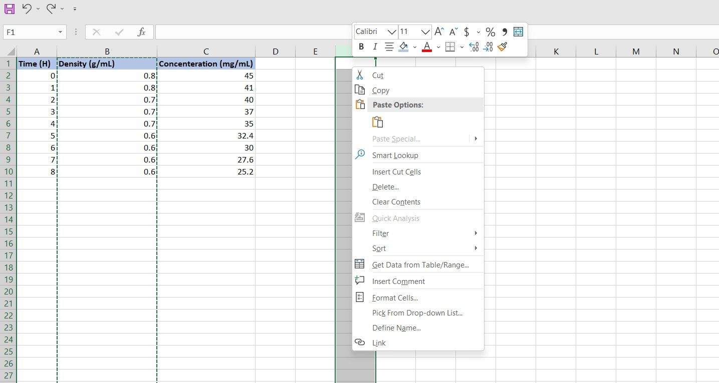
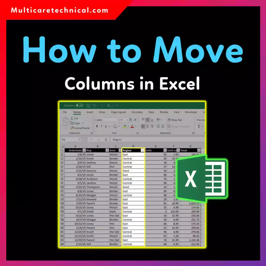
How to move Excel columns can save you a lot of time when rearranging data. Imagine you’ve got a sheet with sales data, but the "Region" column is stuck between "Product" and "Quantity," making it hard to analyze trends. Instead of copying and pasting everything, you can simply drag the column header to its new spot. It’s faster and keeps your formulas intact.
Moving columns isn’t just about aesthetics—it’s about making your data easier to work with. Whether you’re prepping a report or cleaning up a tracker, knowing how to move Excel columns ensures your sheet stays organized. Plus, it’s a skill that pairs well with other Excel tricks, like using tables or conditional formatting, to keep everything tidy.
Rearrange columns for better analysis
If you’re working with a dataset that’s out of order, moving columns is a quick fix. Analysts and project managers benefit most here, especially when dealing with logs or trackers. For example, if you’ve got a sheet tracking tasks with columns like "Priority," "Due Date," and "Status," you might want "Status" front and center for a quick glance.
Set up your sheet with clear headers in row 1 and data starting in row 2. Keep related columns together—like grouping all date fields or all numerical values. This makes it easier to apply filters or sort later. If you’re using a table (Ctrl+T), moving columns within it updates any related formulas automatically.
Here’s a sample task tracker:
| Task ID | Priority | Due Date | Status | Hours Spent |
|---|---|---|---|---|
| 001 | High | 2023-10-15 | Completed | 8 |
| 002 | Medium | 2023-10-20 | In Progress | 4 |
| 003 | Low | 2023-10-25 | Pending | 0 |
To count completed tasks, use =COUNTIFS(Status, "Completed"). This formula returns 1 in this case, since only one task is marked as done.
A common mistake here is merging cells for headers, which breaks the table structure. Always keep headers in a single row and use Center Across Selection from the Alignment tab instead.
Drag and drop with formulas intact
Moving columns with formulas requires a bit of care. If you’ve got a column calculating totals, like =B2C2 for "Total Cost," dragging the column won’t break the formula—Excel updates references automatically. This works best when your sheet uses relative references.
Start by setting up a simple invoice tracker with columns like "Item," "Price," and "Quantity." Add a "Total" column with the formula above. If you move the "Quantity" column, the formula adjusts to =D2E2 if it’s now in column D.
| Item | Price | Quantity | Total |
|---|---|---|---|
| Widget | 10 | 5 | =B2C2 |
| Gadget | 20 | 3 | =B3C3 |
To avoid errors, use =IFERROR(B2*C2, "N/A") in the Total column. This catches any division by zero or missing values, returning "N/A" instead of an error.
One mistake to avoid is hard-coding values. If you type "5" directly into a cell instead of referencing another cell, moving columns won’t update it. Always use cell references for dynamic data.
Use tables for smarter column management
Converting your data range into a table (Ctrl+T) makes moving columns even smoother. Tables automatically adjust formulas and formatting, so you don’t have to worry about breaking anything.
Tables are ideal for logs or checklists where data grows over time. For instance, a project log with columns like "Date," "Task," and "Notes" can be rearranged without messing up filters or totals.
Here’s a sample project log table:
| Date | Task | Notes | Hours |
|---|---|---|---|
| 2023-10-01 | Client Meeting | Follow-up needed | 2 |
| 2023-10-02 | Draft Proposal | Waiting on feedback | 4 |
To sum hours, use =SUM(Table1[Hours]). If you move the "Hours" column, the formula still works because tables use structured references.
A common pitfall is forgetting to expand the table when adding new columns. Always click the table, go to Table Design > Resize Table, and update the range to include new data.
Fix broken references after moving
Even with careful planning, moving columns can sometimes break formulas. If you’ve got a VLOOKUP or XLOOKUP referencing a column you moved, you’ll need to update the formula manually.
For example, if your lookup formula references column C but you moved it to column E, change =XLOOKUP(A2, C:C, D:D) to =XLOOKUP(A2, E:E, F:F).
| ID | Name | Department | Manager |
|---|---|---|---|
| 1 | John | Sales | =XLOOKUP(C2, E:E, F:F) |
| 2 | Jane | Marketing | =XLOOKUP(C3, E:E, F:F) |
To prevent this, use named ranges or tables. Go to Formulas > Define Name, select the range, and give it a name like "Departments." Then use =XLOOKUP(A2, Departments, Managers)—this stays intact even if columns move.
One mistake is not checking for numbers stored as text. If a column with numerical data is formatted as text, formulas might not work after moving. Use Data > Text to Columns to convert it back to numbers.
Try moving a column in your own sheet and adding a conditional formatting rule to highlight values above a certain threshold. It’s a quick way to see how changes affect your data.