






Setting Up Your Data for Success
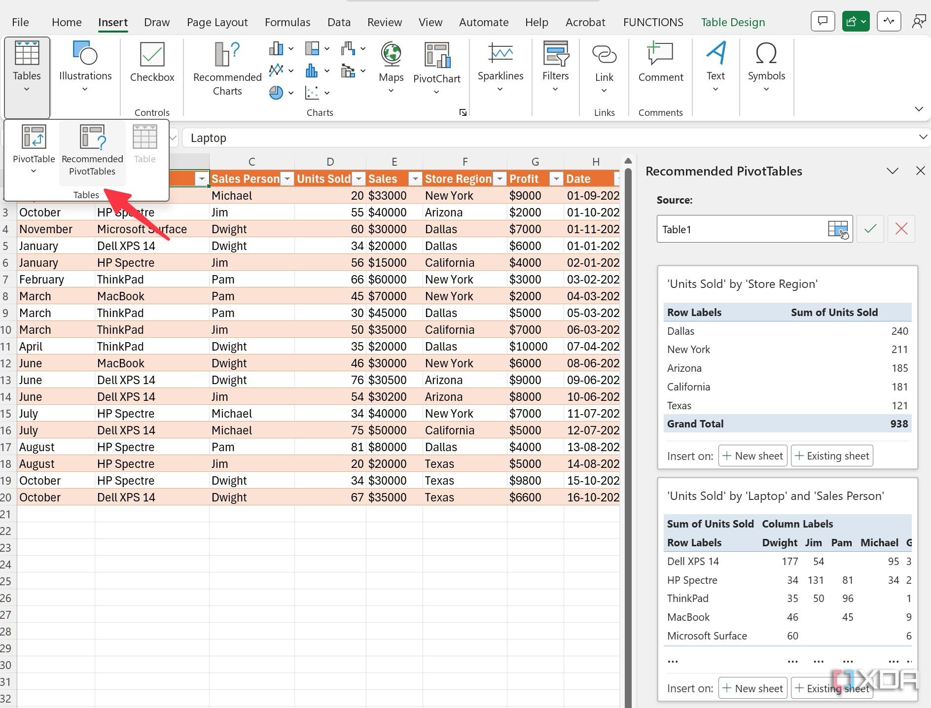
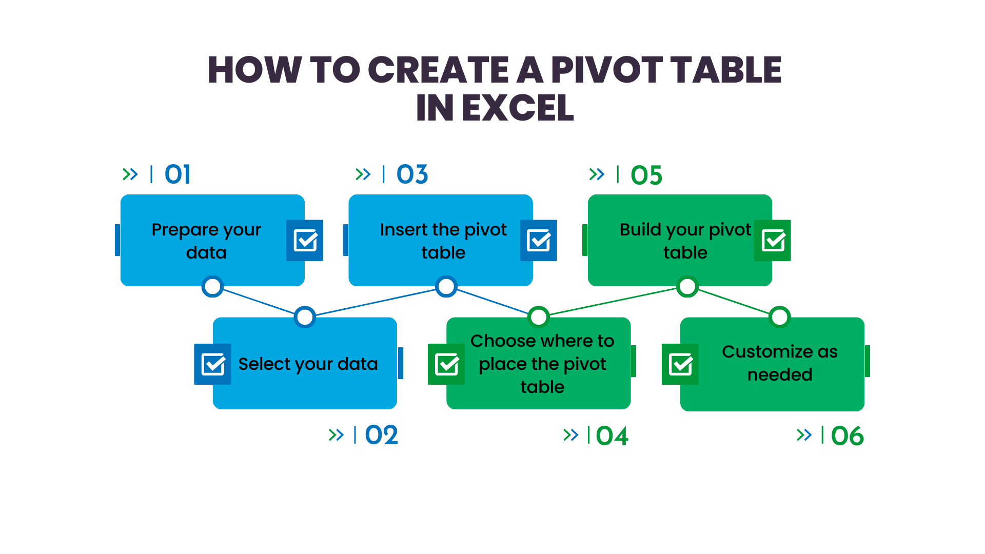
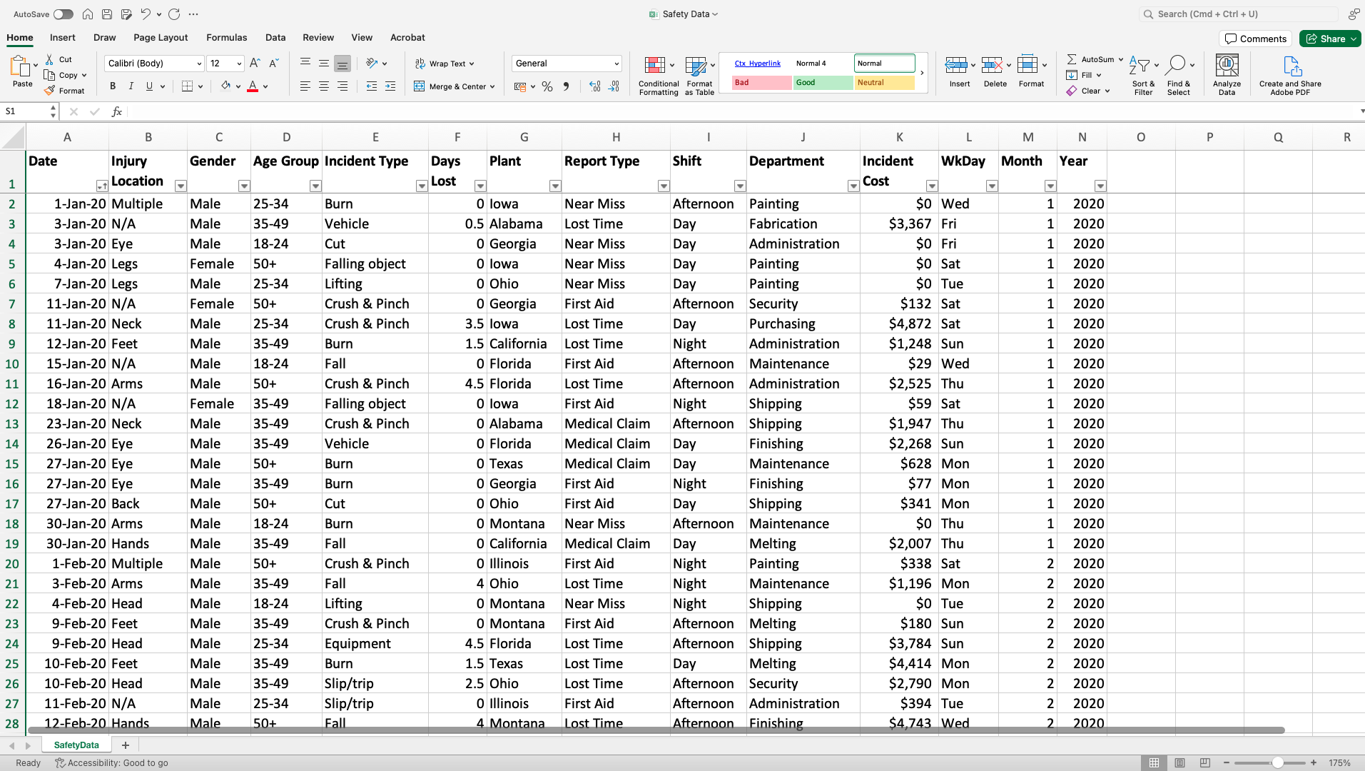
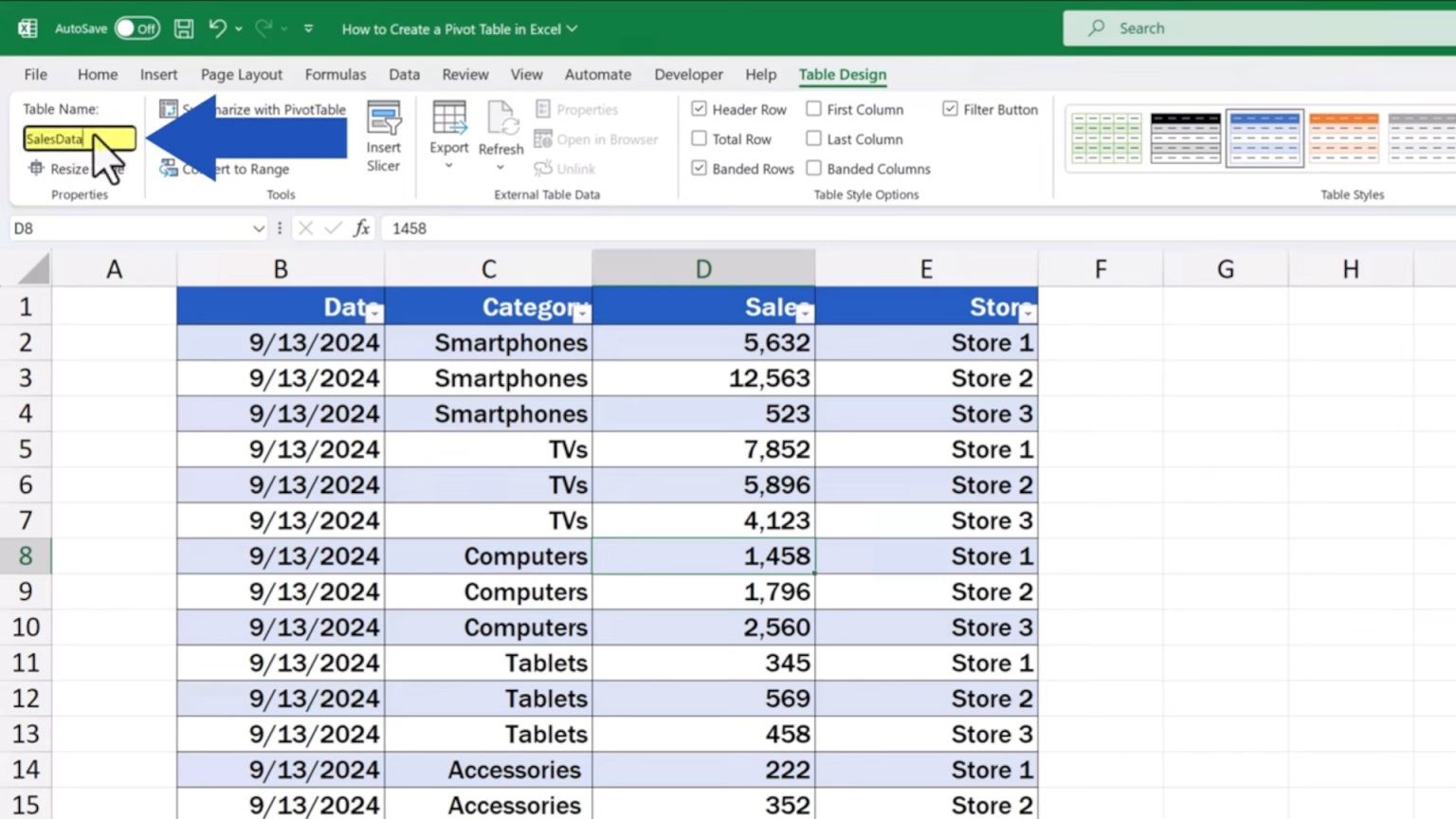
When it comes to creating pivot charts, the first step is ensuring your data is structured properly. Think of your spreadsheet as a house; the columns are the rooms, and the rows are the items within each room. So, before we start, let's tidy up our data: make sure your columns have clear, concise headers, and your rows are consistent and organized. This step is crucial because it lays the foundation for an accurate and effective pivot chart.
Now, let's talk about the tools Excel provides to make this process smoother. Excel has some fantastic built-in features to help with data manipulation and formatting. For instance, you can use the XLOOKUP formula to quickly find and retrieve specific data points, or the IF function to create conditional rules for your data. These formulas are your friends and can save you a lot of time and effort, especially when dealing with large datasets.
Building Your Pivot Chart
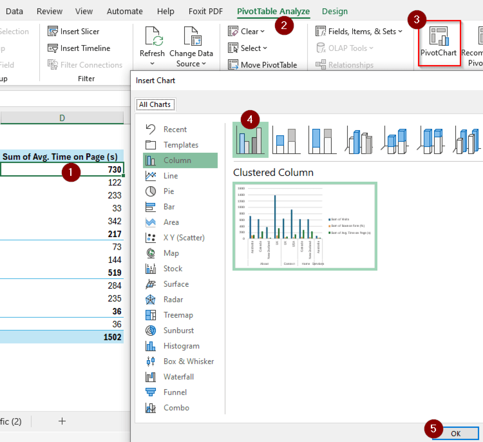
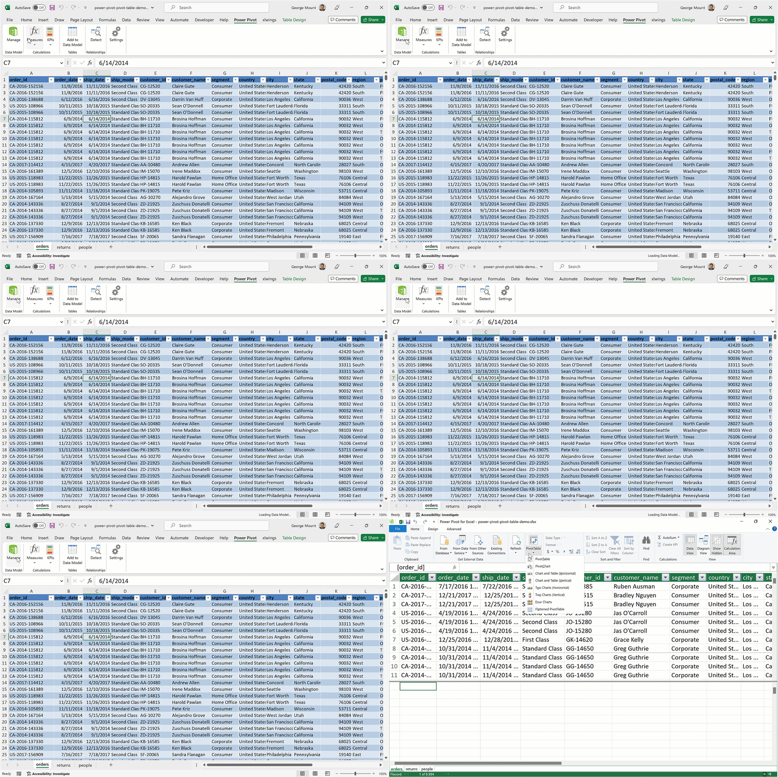
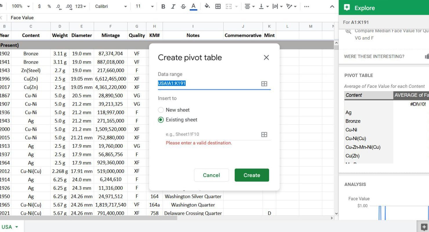
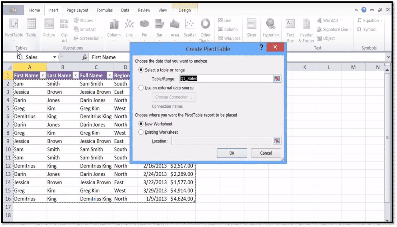
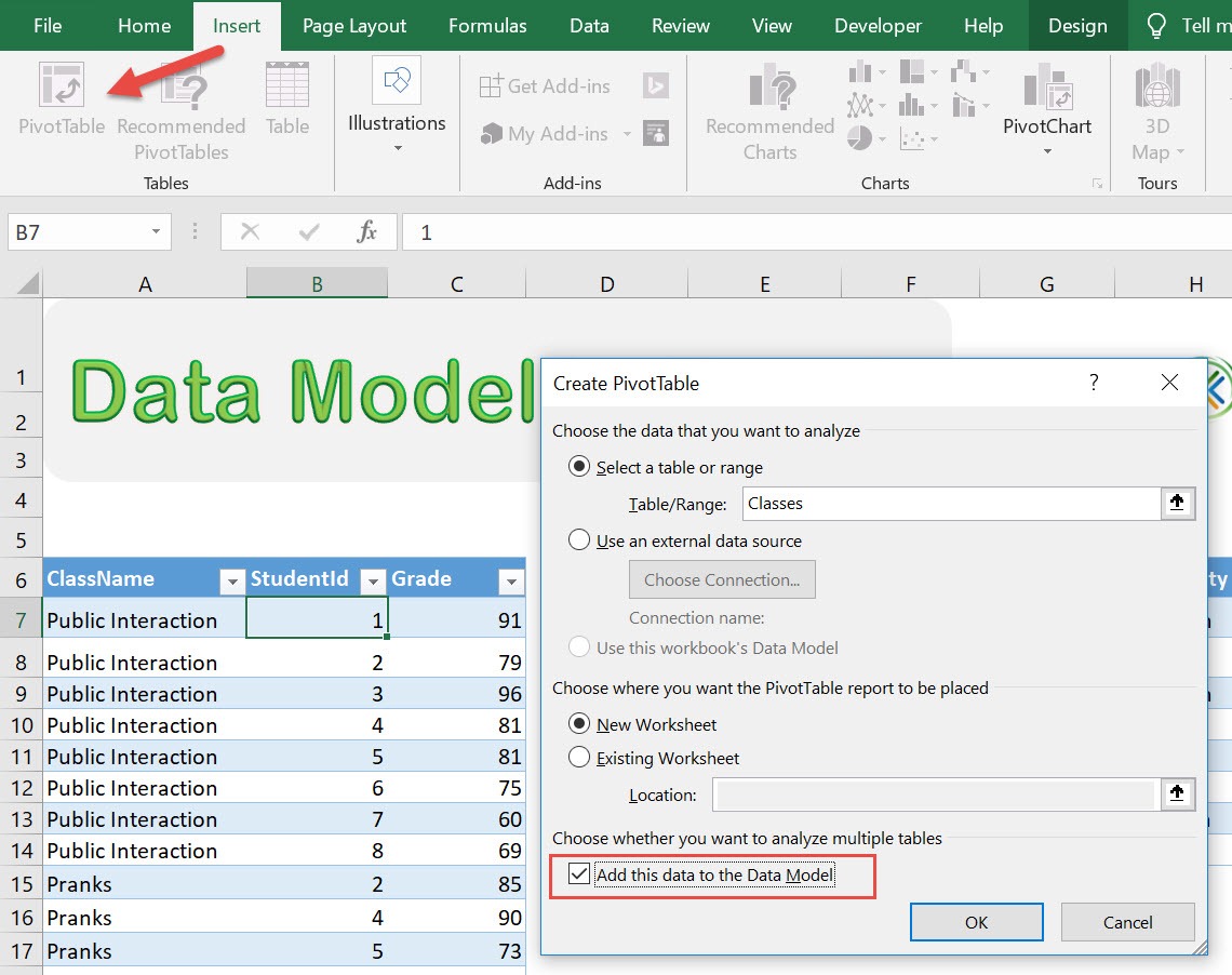
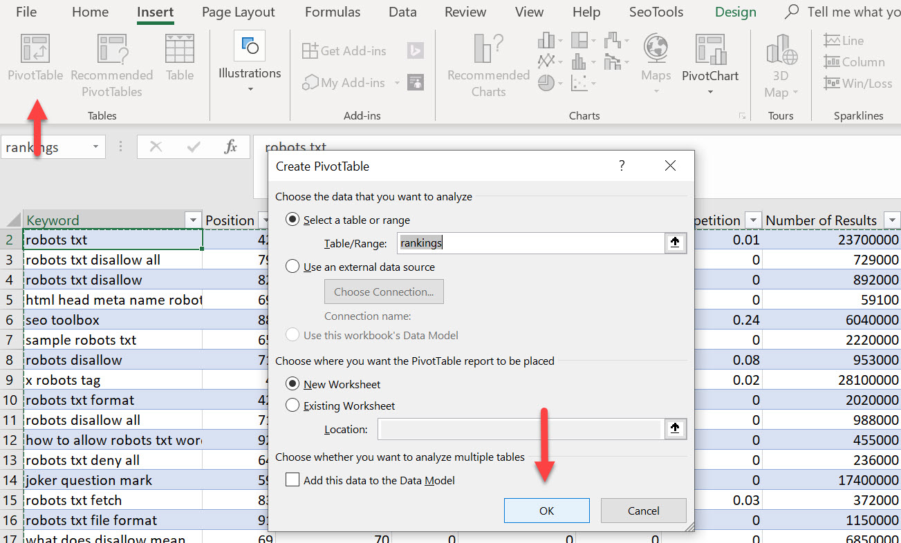
Once your data is shipshape, it's time to build your pivot chart. Excel makes this process pretty straightforward. Go to the Insert tab and select PivotChart. From here, you'll be prompted to choose the data range you want to include in your chart. Excel will then display a new window where you can customize your chart's layout.
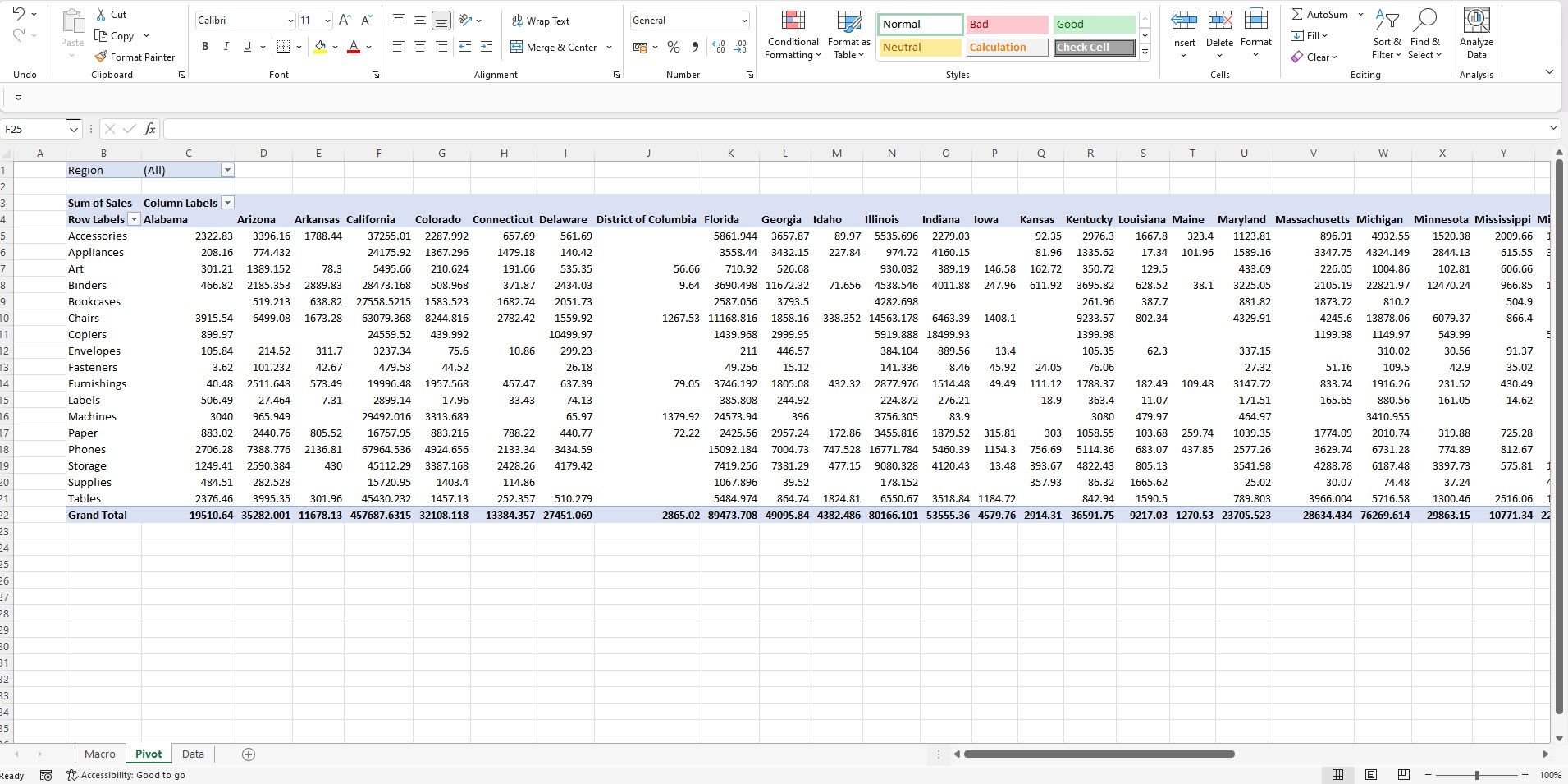
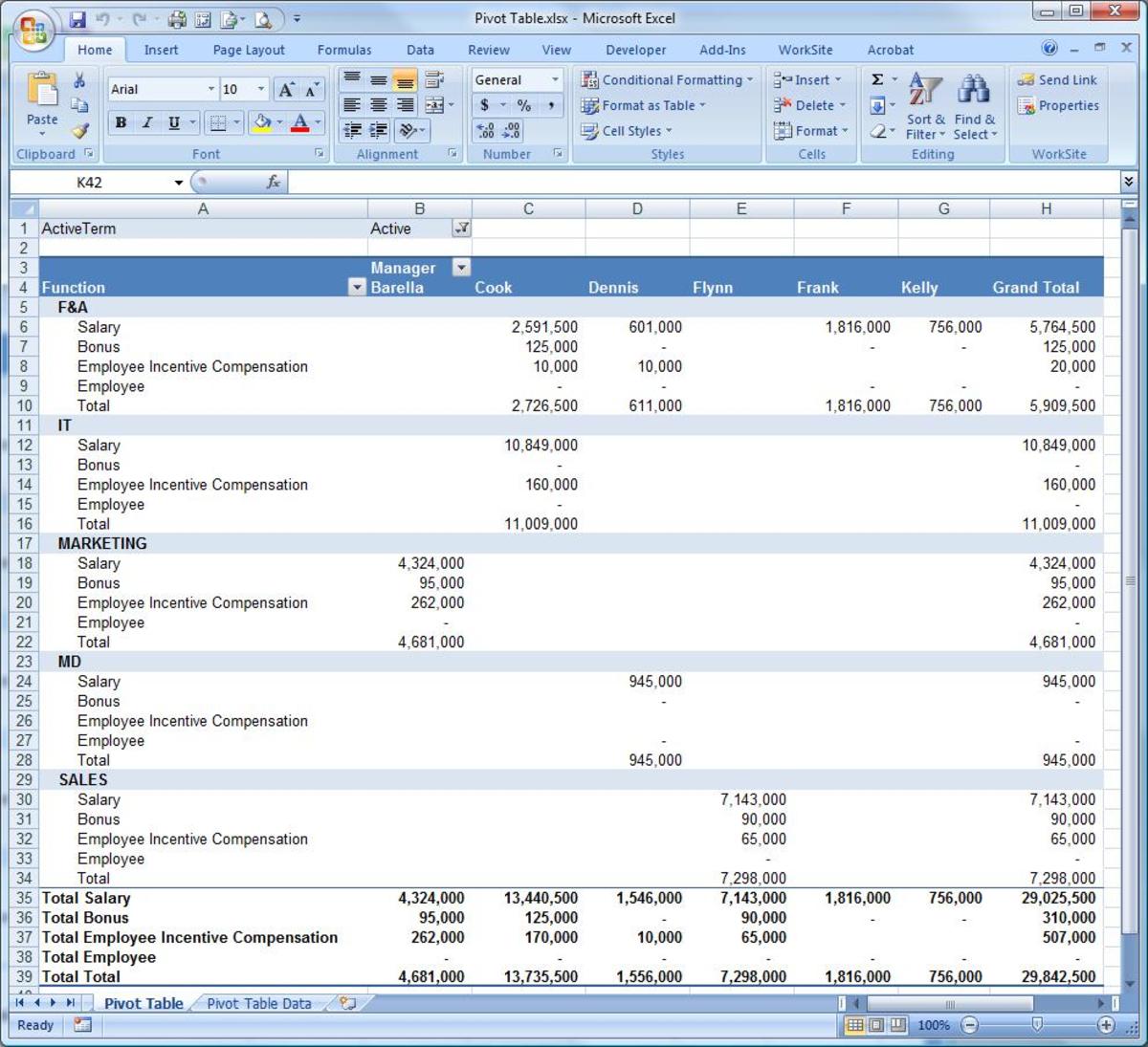
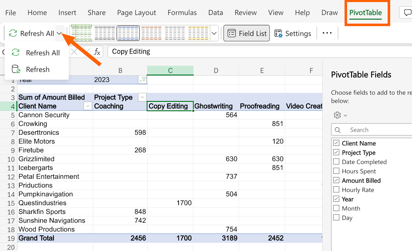
This is where the magic happens! You can drag and drop fields to create rows, columns, and even filters for your chart. For example, if you have a dataset with sales data, you could drag the "Product" field to the Rows area, and the "Sales Amount" field to the Values area. This will create a chart that shows the sales performance of each product.
Customizing and Refining
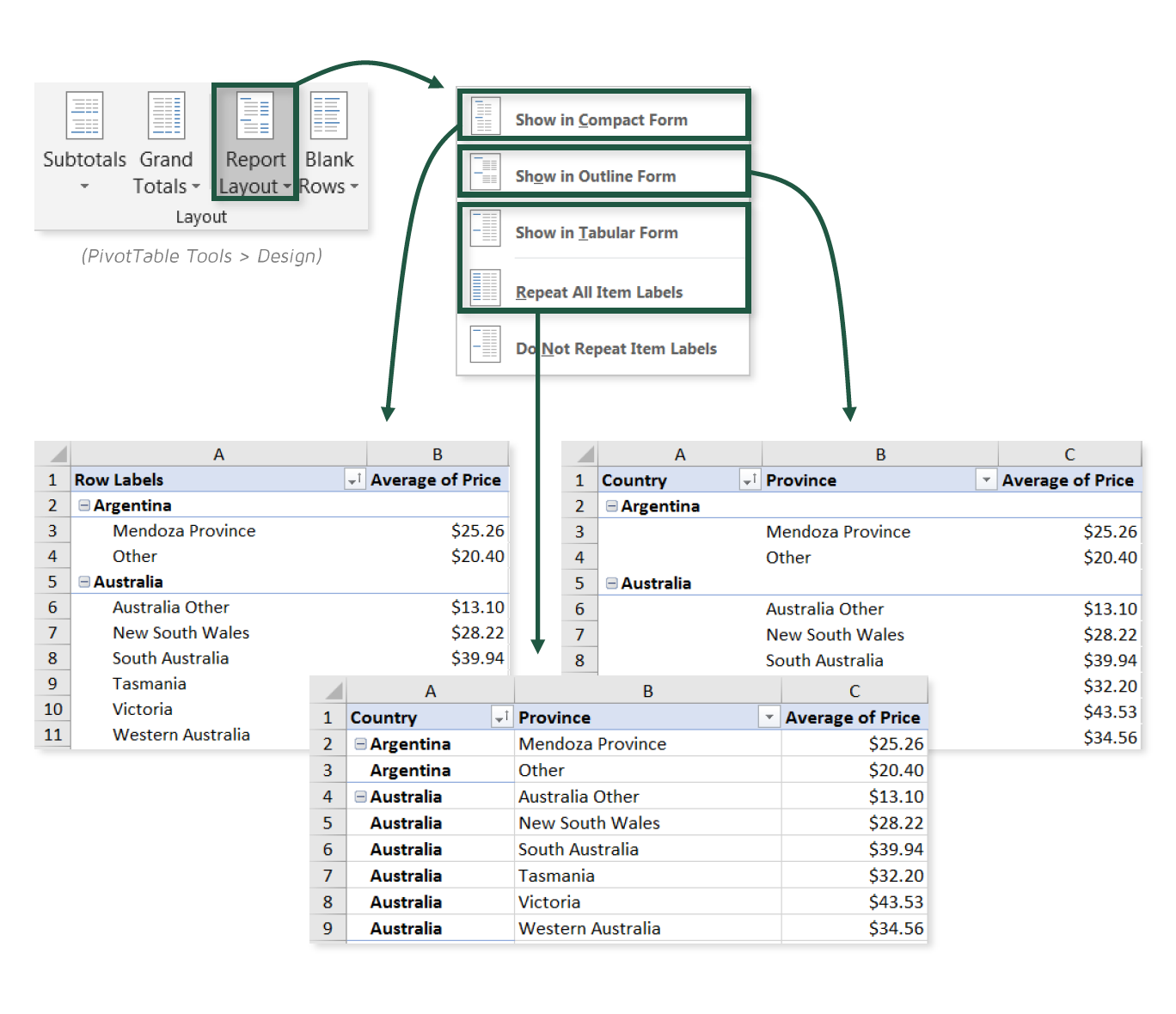
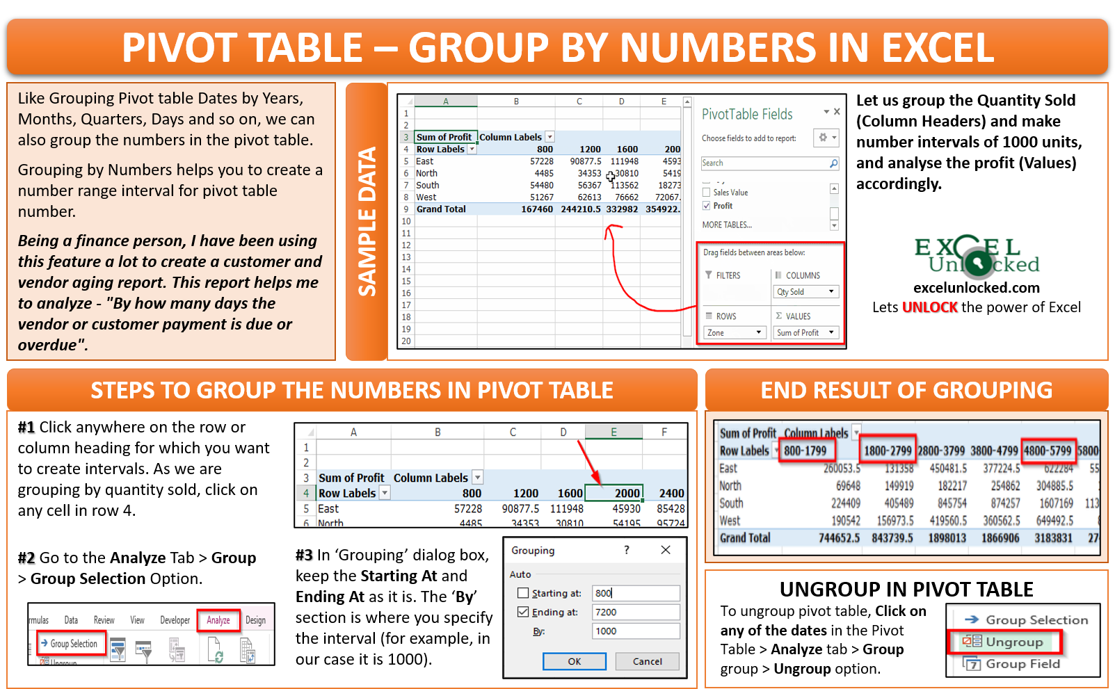
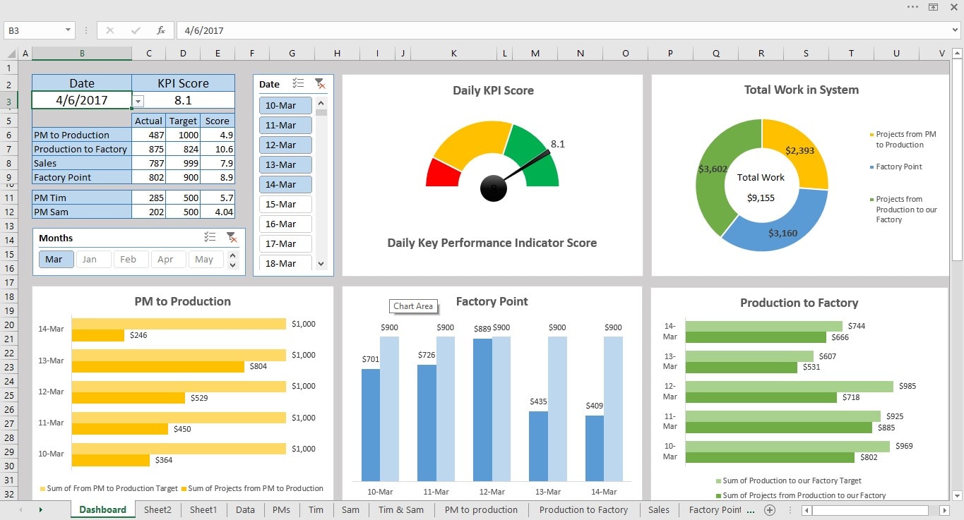
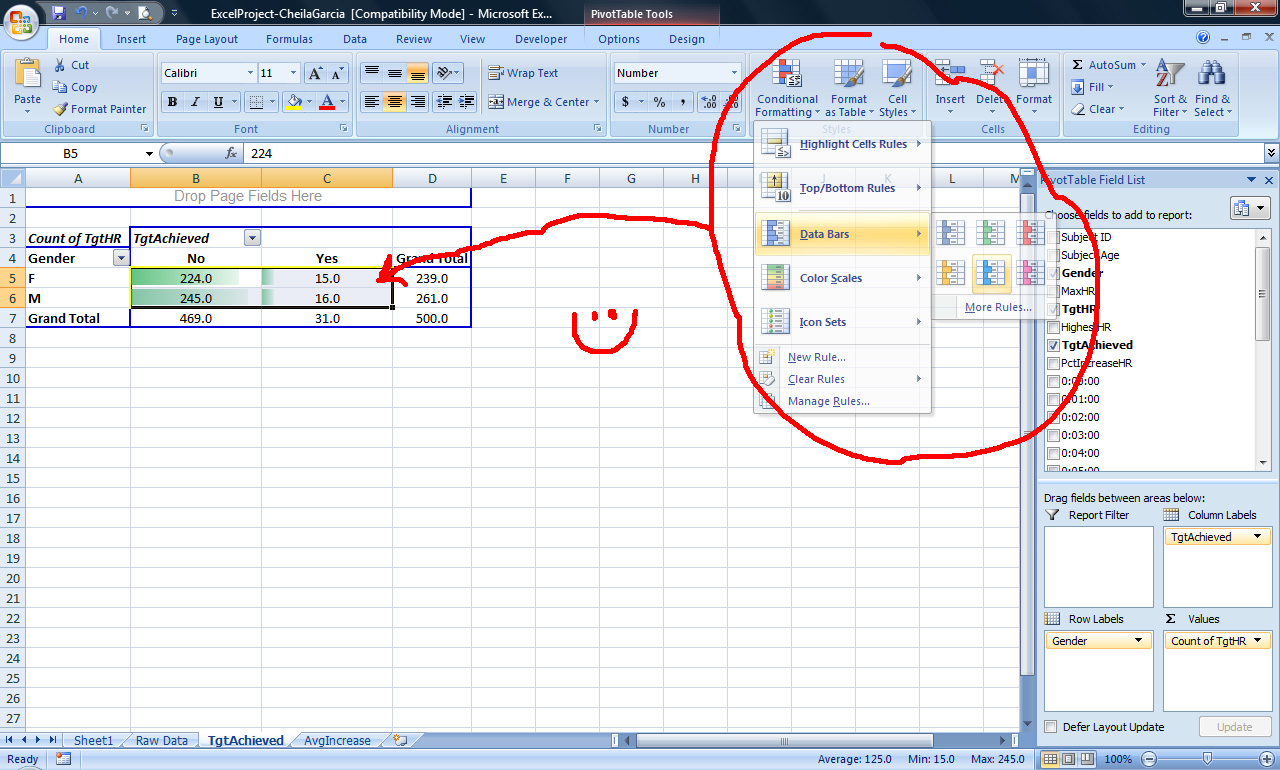
Now that you have your basic pivot chart, it's time to add some polish. Excel offers a range of customization options to make your chart truly shine. You can change the chart type, add titles and labels, and even apply conditional formatting to highlight specific data points. For instance, you could use conditional formatting to highlight cells with sales above a certain threshold, making it easy to identify top-performing products at a glance.
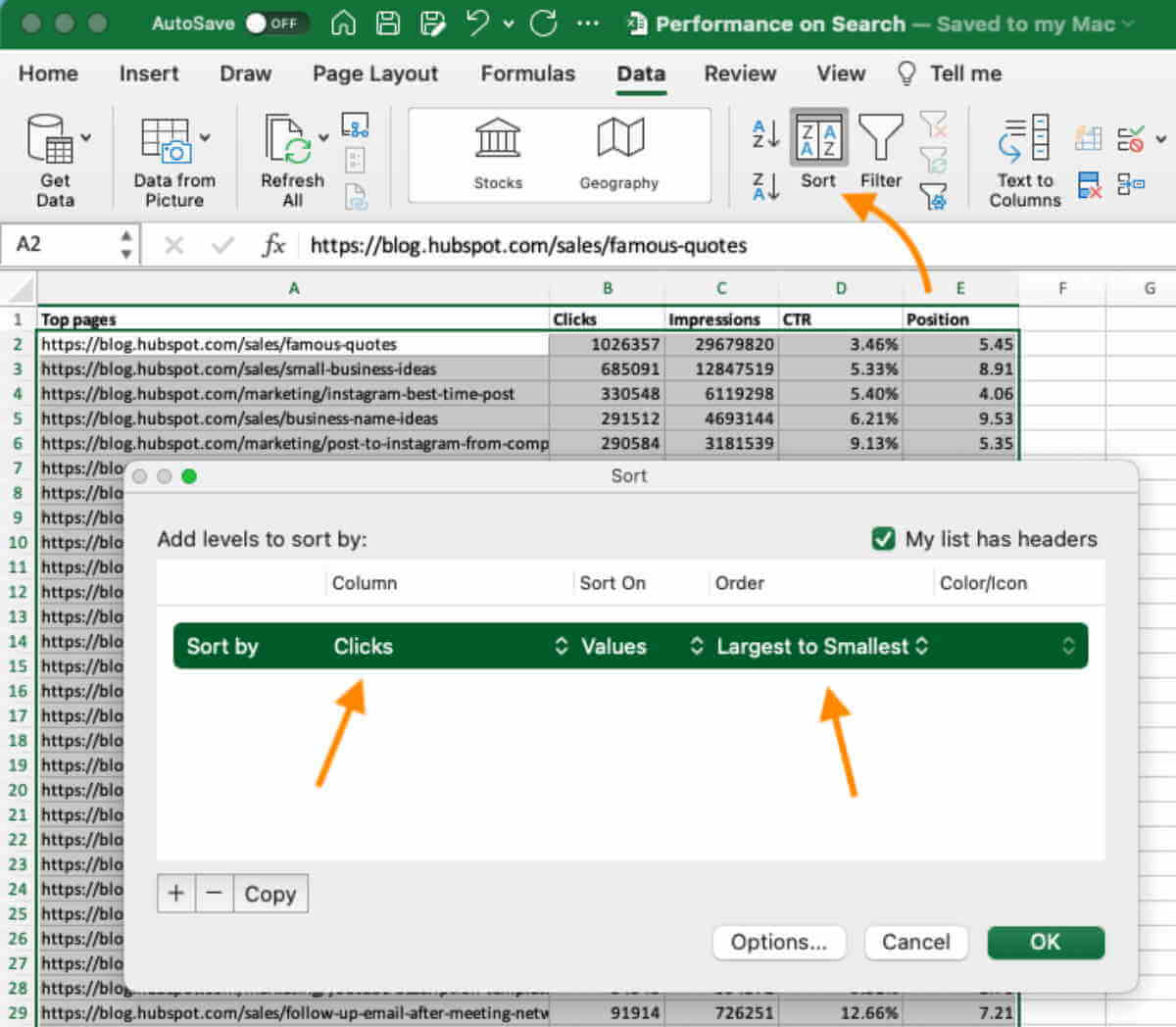
Another useful feature is the ability to create drop-down lists in your pivot chart. This allows you to quickly filter your data by selecting different options from a drop-down menu. It's a great way to make your chart more interactive and user-friendly.
Final Thoughts
So, there you have it! Creating pivot charts in Excel is a powerful way to visualize and analyze your data. It might seem a bit daunting at first, but with a bit of practice and familiarity with Excel's tools, you'll be creating dynamic charts in no time.
Next time you open a spreadsheet, why not give it a go? You might just discover a whole new way to understand and present your data.