





Hyperscale Data Center Construction Blank Overview
A 1-100 chart is a simple way to show numbers from one to one hundred in Excel. This post shows how to create it quickly using Excel fill series and a bar chart.
You can use the auto‑fill handle to generate the numbers, then turn the range into a chart with a few clicks. The exact steps can vary a bit depending on your Excel version, but the core idea stays the same.
Excel online guide: Create a 1‑100 chart with fill series and a bar chart
If you need a quick visual of the numbers from one to one hundred, a 1-100 chart is the simplest solution in Excel. You can generate the numbers automatically and turn them into a bar chart without any coding.
Start by using Excel auto fill numbers to populate a column with the sequence 1, 2, 3… up to 100. Select the filled range, then insert a bar chart to see each value as a bar.
The process works the same in recent versions such as Microsoft 365 Excel, Excel 2019, and Excel for the web, so you don’t need to worry about version differences.
Data range setup: What must be true first
Before you begin, make sure Excel is not in protected view and that the worksheet is not protected, otherwise fill commands will be disabled.
A clear range helps Excel data visualization tools work correctly. If you are on a corporate account, confirm that macros or add‑ins are not blocked by policy.
If you are using Excel on the web, ensure you have edit permissions for the file; a read‑only view will prevent the fill handle from working.
If you convert the filled range into an Excel table (Ctrl+T), the fill handle will automatically extend when you add new rows, and the chart will reference the entire table without manual range updates.
Fill series steps: How to generate numbers and build the chart
Follow these steps to create the numbers and the chart in a few minutes.
- Select cell A1 and type 1, then click the fill handle (small square at the corner) and drag down while holding the left mouse button to extend the series.
- Release the mouse and choose Fill Series from the AutoFill options that appear; this tells Excel to continue the numeric sequence.
- With the column selected, go to the Insert tab and choose 2-D Column from the Charts group to create a bar chart based on the data.
- Excel will place the chart on the sheet; click the chart to select it and use the Chart Design tab to adjust titles and axis labels if needed.
- If you want the chart to reflect the full 1-100 chart, make sure the data range includes cell A100; you can resize the selected area manually or let Excel auto‑detect the range.
- To improve readability, add a chart title like “Numbers 1‑100” and label the vertical axis as “Value”.
- Finally, save the workbook; the chart will update automatically if you later extend the fill series beyond 100.
Chart design basics: Why it may not work and what to check
Sometimes the chart appears blank, shows wrong values, or the fill series stops early; checking a few items usually fixes it.
- Make sure the fill handle was dragged correctly and the AutoFill option selected; without it Excel treats the numbers as plain text.
- Verify that the cells are formatted as General or Number; a custom format that hides values can cause the chart to be empty.
- Check that the chart’s data source range matches the filled column; a mismatched range can show only part of the sequence.
- Ensure the workbook is not in read‑only mode and that you have edit permission; otherwise Excel won’t update the chart.
After making any corrections, save the file and reopen it to confirm the chart displays the full sequence; a fresh open often resolves display glitches.
Axis labels adjust: A safer way to avoid problems next time
A more robust method is to create an Excel table for the numbers; when you add a new row, the table expands and the chart updates automatically.
You can also define a named range that uses the OFFSET function to grow as you fill, then base the chart on that named range instead of a fixed address.
If you prefer not to use a table, generate the numbers with a simple formula such as =ROW()-ROW($A$1)+1 in each cell; the chart will still reflect the 1-100 chart as long as the formula fills down.
Finally, keep axis labels simple and avoid merging cells; merged cells can interfere with chart selection and cause unexpected behavior.
Another option is to use a sparkline in a cell next to the numbers; it provides a compact visual of the trend without taking up sheet space, and it updates automatically as you fill.
Quick note: the menu names can look a bit different depending on your version of Excel, so don’t be surprised if something shows up in a different spot.
If you found this helpful, feel free to browse the other Microsoft Office guides on the site whenever you need a quick tip or a fix.
Related: Hyperscale Data Center Construction Essential Guide
Hyperscale data center construction is an impressive feat of engineering, but it's not something you see every day. These massive facilities are like hidden powerhouses, quietly keeping our digital world running. So, what's the story behind these data centers, and why should we care?
Understanding Hyperscale Data Centers
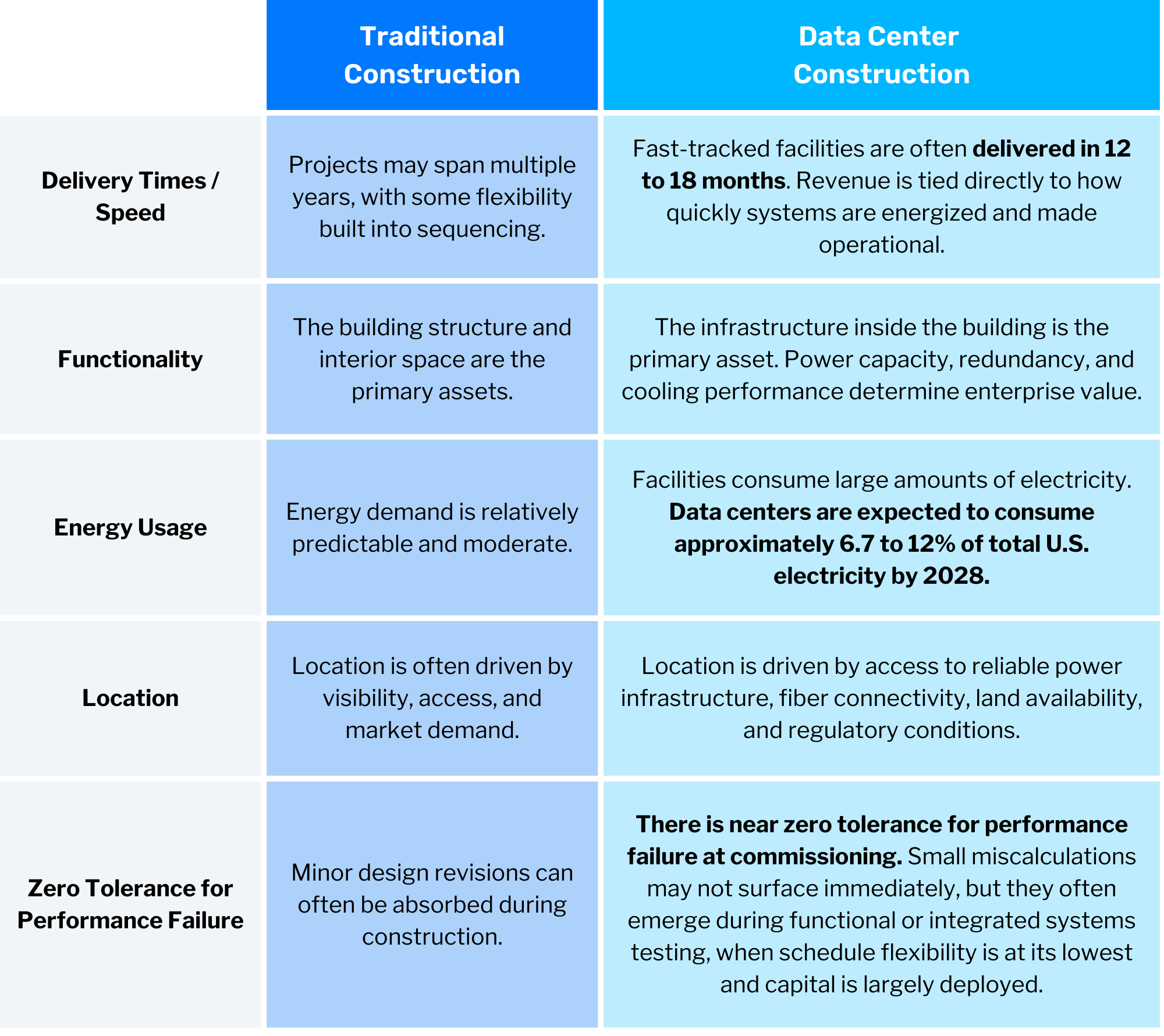
Hyperscale data center construction is all about creating enormous data storage and processing facilities. These centers are designed to handle vast amounts of data and provide the computing power needed for modern businesses and technologies. They're not just big; they're built to be efficient, secure, and reliable. From cloud services to streaming platforms, these centers keep our digital lives humming.
The construction process is complex. It involves careful planning, site selection, and the use of specialized materials and equipment. Everything from the foundation to the cooling systems must be designed to handle the unique demands of data storage and processing. It's a delicate balance of engineering and technology.
The Practical Side of Construction
When it comes to building these centers, several key factors come into play. The first is the location. Finding the right site is crucial. It needs to have access to power, water, and good transportation links, and it should also consider the local climate and any potential natural hazards.
Then there's the design and construction process itself. This involves a lot of specialized knowledge and coordination. Architects, engineers, and construction teams work together to create a facility that meets all the technical requirements. This includes everything from the structural design to the installation of complex cooling systems and power distribution networks.
Costs and Considerations
The cost of hyperscale data center construction is significant, but it varies widely depending on the size, location, and specific requirements. It's not just about the building itself; you also need to consider the ongoing operational costs, like power and maintenance. These centers are energy-intensive, so efficient design and the use of renewable energy sources can make a big difference.
When comparing quotes, it's important to look beyond the initial construction costs. Consider the long-term viability and the potential for future expansion. A good quote should cover all aspects, from site preparation to the final fit-out, and provide a clear breakdown of costs.
The Role of Construction Companies
Large construction firms often take on hyperscale data center construction projects. These companies have the expertise, resources, and specialized teams needed for such complex builds. They can handle everything from initial planning to project management and construction.
When hiring a company for such a project, it's crucial to check their experience and track record. Look for companies that have successfully completed similar projects and have a good reputation. Ask for references and case studies to get a sense of their capabilities and the quality of their work.
Final Thoughts
Hyperscale data center construction is an intriguing aspect of modern infrastructure. It combines cutting-edge technology with traditional construction skills. While it's not something most of us will undertake, understanding the process gives us a glimpse into the digital world we rely on daily. It's a fascinating blend of old and new, and a reminder of the incredible engineering feats happening behind the scenes.
Related: match formula excel easy guide for data lookups
Match formula Excel can save you hours when you need to find something in a long list. Say you’ve got a sheet with hundreds of product IDs, and you need to know the position of a specific one. Instead of scrolling forever, you type in =MATCH(lookup_value, lookup_array, [match_type]), and Excel does the heavy lifting. It’s not just for numbers—it works with text, dates, and even wildcards if you set it up right.
It’s one of those formulas that feels like a secret weapon once you get the hang of it. Sure, XLOOKUP is flashier, but match formula Excel is faster for grabbing a position, not a value. Plus, it plays well with INDEX for more advanced lookups. If you’re still manually searching for data, this is your cue to stop.
Find positions, not just values
The match formula in Excel is all about locating where something sits in a list. It’s perfect for anyone who needs to map data between sheets or check if an item exists. Marketers use it to match campaign IDs to results, inventory managers track stock locations, and HR teams map employee IDs to departments.
Set up your sheet with two columns: one for your lookup list (e.g., product IDs) and one for the data you’re matching against (e.g., sales numbers). Keep the lookup list sorted if you’re using match_type 1 (exact or next smallest). Add a third column for the formula itself, and a fourth for any error handling with IFERROR.
| Product ID | Sales | Position | Formula |
|---|---|---|---|
| 101 | 250 | =MATCH(101, A2:A100, 0) |
|
| 102 | 300 | =MATCH(103, A2:A100, 1) |
|
| 103 | 150 | =MATCH("104", A2:A100, 0) |
The first formula returns 1 because 101 is the first item in the list. The second returns 5 since 103 isn’t there, but 105 is the next smallest. The third returns #N/A because "104" (as text) doesn’t match 104 (as a number).
Common mistake: Using match_type 1 on unsorted data. Excel won’t throw an error, but it’ll give you wrong results. Fix it by sorting the lookup array or switching to match_type 0 for exact matches.
Pair it with INDEX for dynamic lookups
The real power of match formula Excel comes when you combine it with INDEX. Together, they let you pull values from a table based on a lookup, without hard-coding cell references. This is how you build dynamic dashboards or reports that update automatically.
Create a table with Ctrl+T, then add a separate cell for your lookup value (e.g., "Q1 Sales"). Below it, set up a formula like =INDEX(table_array, MATCH(lookup_value, lookup_column, 0), return_column). Use IFERROR around it to catch missing data.
| Quarter | Region | Sales | Formula |
|---|---|---|---|
| Q1 | East | 500 | |
| Q1 | West | 700 | |
| Q2 | East | 600 |
Formula in D2: =IFERROR(INDEX(B2:B4, MATCH("Q1", A2:A4, 0), 2), "Not Found"). Returns 500 for Q1 East sales.
Common mistake: Forgetting to lock cell references with $. If you drag the formula down, A2:A4 should be $A$2:$A$4 to keep it anchored.
Handle errors and wildcards
Match formula in Excel breaks if it can’t find what you’re looking for. Wrap it in IFERROR to show a custom message instead of #N/A. If you’re working with partial matches, use wildcards by switching to match_type 0.
Add a data validation dropdown in your lookup cell to avoid typos. Go to Data > Data Validation > List, and point it to your lookup array. This keeps inputs consistent.
| Item | Price | Lookup | Result |
|---|---|---|---|
| Apple | 1.50 | p | 1 |
| Banana | 0.75 | n | 2 |
| Cherry | 2.00 | Peach | Not Found |
Formula in D2: =IFERROR(MATCH(C2 & "", A2:A4, 0), "Not Found"). For p, it returns 1 because "Apple" contains “p”.
Common mistake: Storing numbers as text. If your lookup value is 101 (number) but your array has "101" (text), the formula fails. Fix it with Data > Text to Columns > Finish to convert.
Build a lookup tracker
Turn match formula Excel into a reusable tracker by adding conditional formatting and filters. This works great for inventory logs, expense trackers, or project checklists. Highlight matches with Home > Conditional Formatting > New Rule > Use a formula.
Set up a filter on your lookup column (Ctrl+Shift+L) so you can narrow down results. Freeze the top row (View > Freeze Panes) if your sheet is long.
| Task ID | Status | Due Date | Priority |
|---|---|---|---|
| 001 | Done | 2023-10-15 | High |
| 002 | Pending | 2023-10-20 | Medium |
| 003 | Done | 2023-10-25 | Low |
Formula in E2: =IF(ISNUMBER(MATCH(A2, $A$2:$A$4, 0)), "Found", ""). Add conditional formatting to highlight “Found” cells.
Common mistake: Merging cells in your lookup array. Merged cells break formulas. Unmerge them with Home > Merge & Center > Unmerge Cells.
Try building a simple inventory tracker next. Use match formula Excel to flag low-stock items, and pair it with COUNTIFS to tally quantities.