













Find positions, not just values
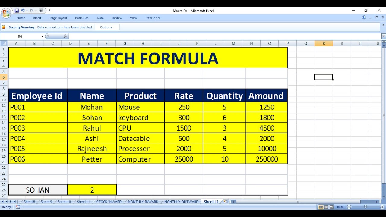
The match formula in Excel is all about locating where something sits in a list. It’s perfect for anyone who needs to map data between sheets or check if an item exists. Marketers use it to match campaign IDs to results, inventory managers track stock locations, and HR teams map employee IDs to departments.
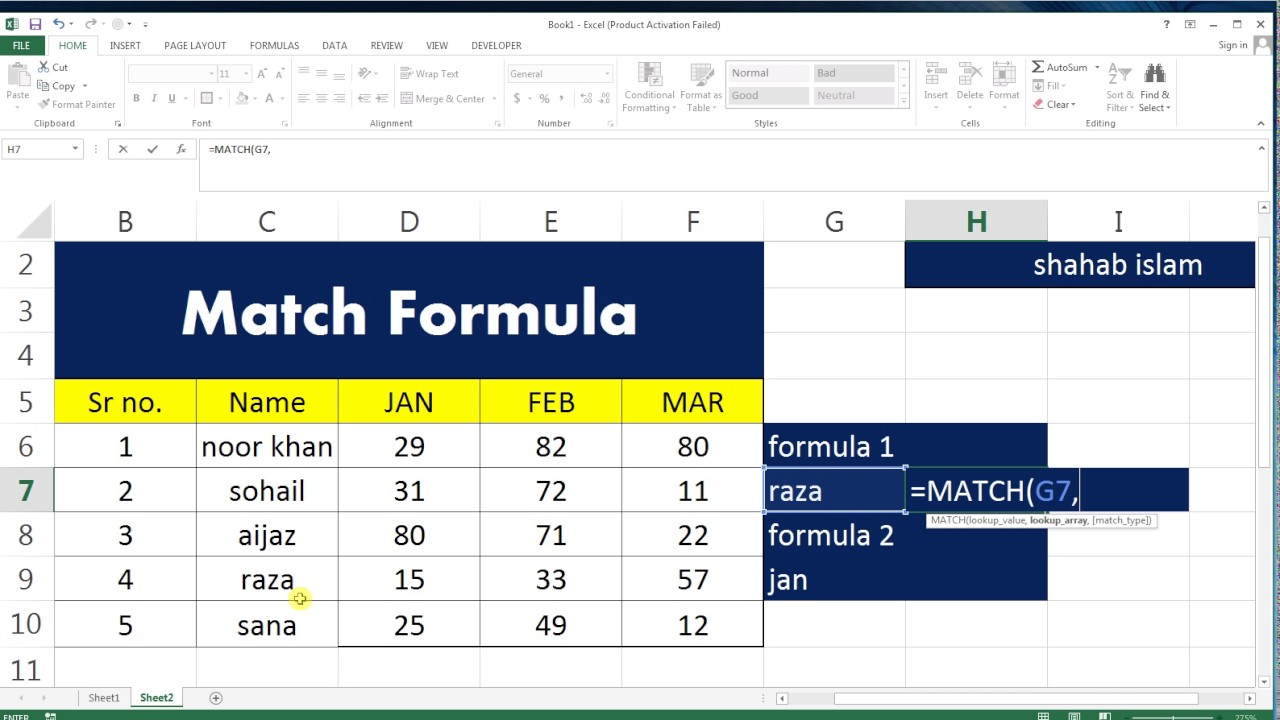
Set up your sheet with two columns: one for your lookup list (e.g., product IDs) and one for the data you’re matching against (e.g., sales numbers). Keep the lookup list sorted if you’re using match_type 1 (exact or next smallest). Add a third column for the formula itself, and a fourth for any error handling with IFERROR.
| Product ID | Sales | Position | Formula |
|---|---|---|---|
| 101 | 250 | =MATCH(101, A2:A100, 0) |
|
| 102 | 300 | =MATCH(103, A2:A100, 1) |
|
| 103 | 150 | =MATCH("104", A2:A100, 0) |
The first formula returns 1 because 101 is the first item in the list. The second returns 5 since 103 isn’t there, but 105 is the next smallest. The third returns #N/A because "104" (as text) doesn’t match 104 (as a number).
Common mistake: Using match_type 1 on unsorted data. Excel won’t throw an error, but it’ll give you wrong results. Fix it by sorting the lookup array or switching to match_type 0 for exact matches.
Pair it with INDEX for dynamic lookups
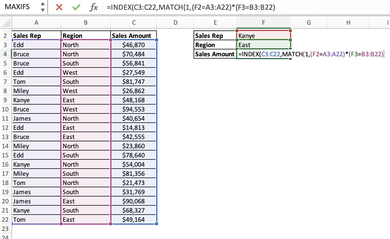
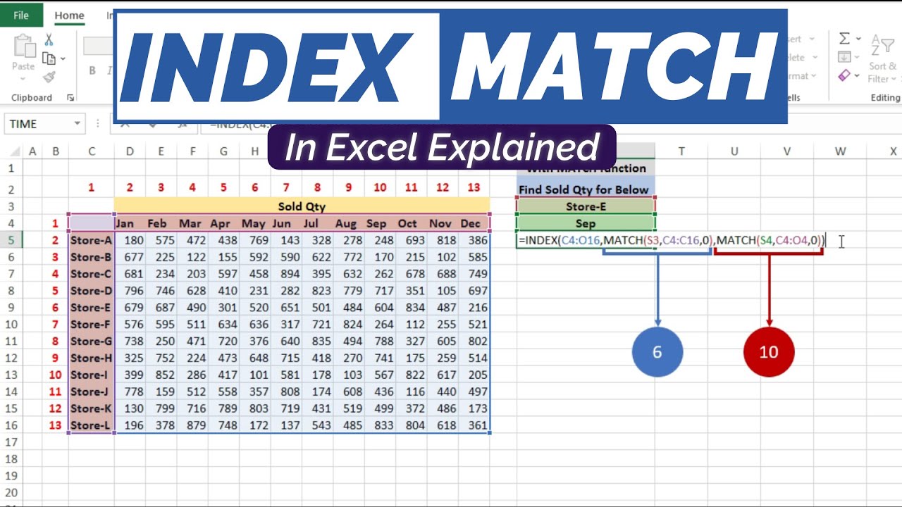
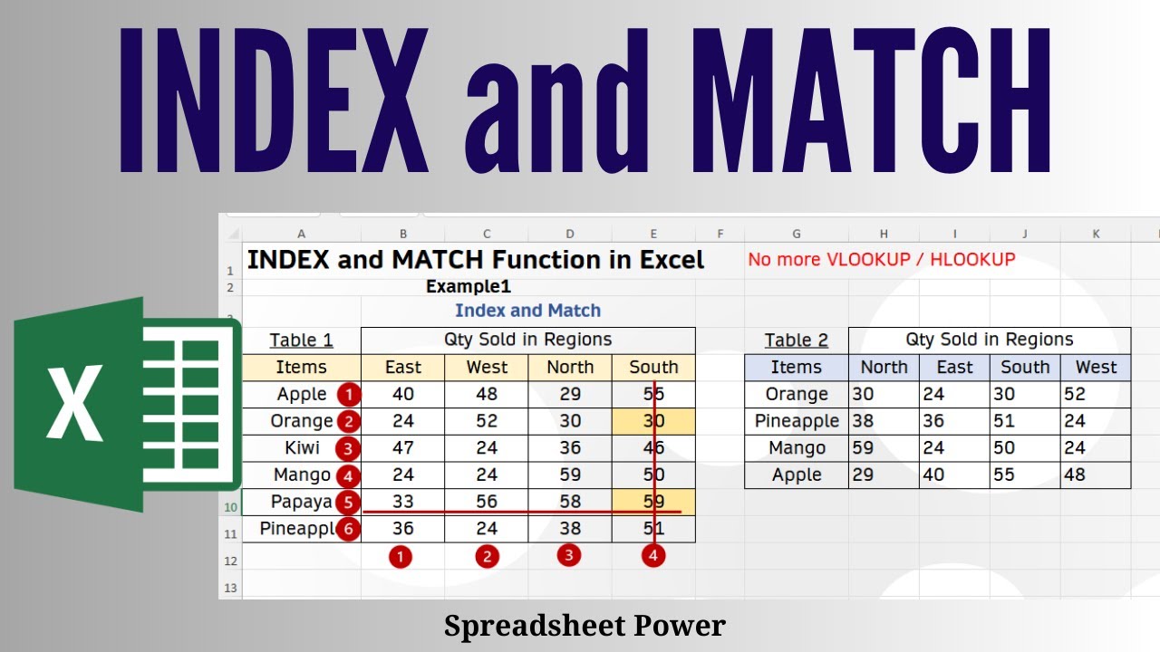
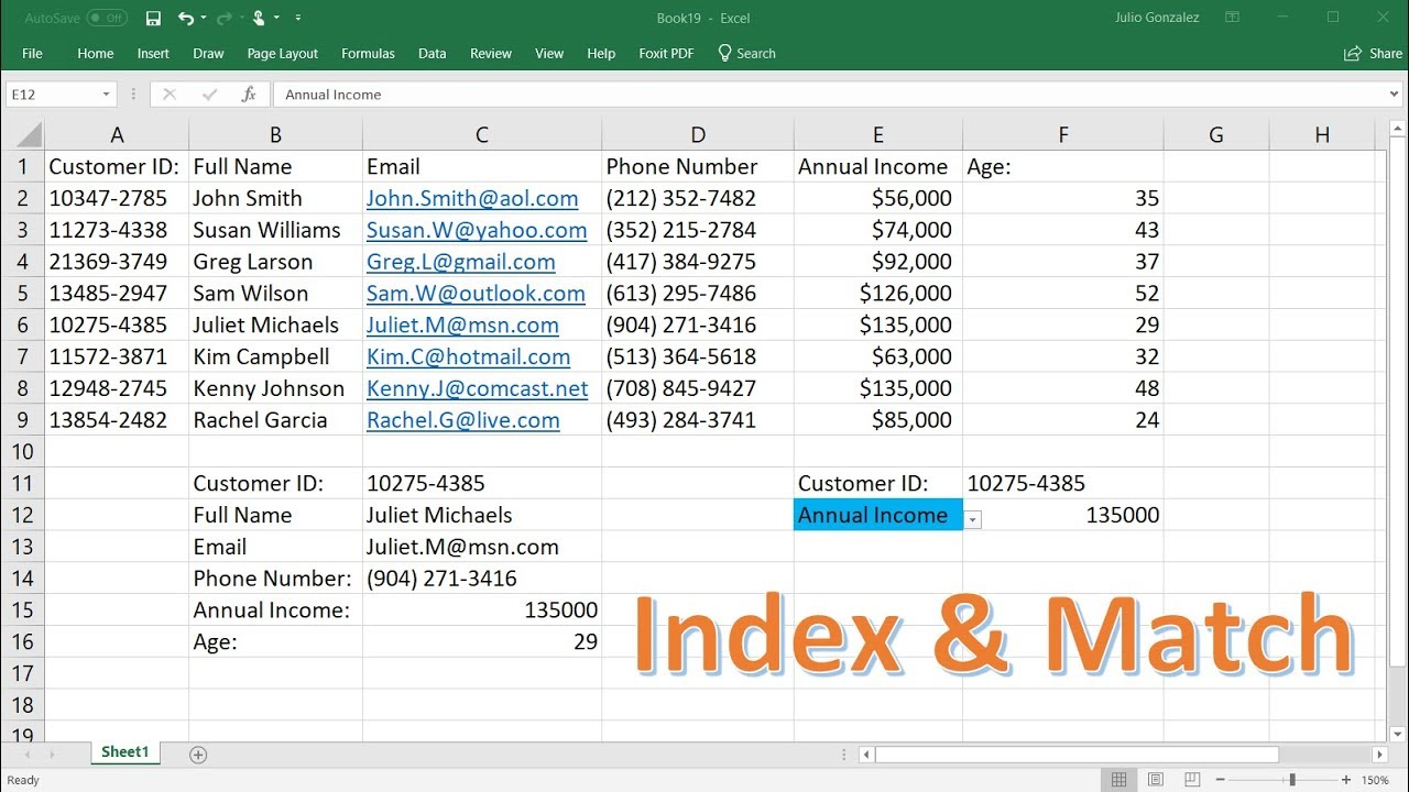
The real power of match formula Excel comes when you combine it with INDEX. Together, they let you pull values from a table based on a lookup, without hard-coding cell references. This is how you build dynamic dashboards or reports that update automatically.
Create a table with Ctrl+T, then add a separate cell for your lookup value (e.g., "Q1 Sales"). Below it, set up a formula like =INDEX(table_array, MATCH(lookup_value, lookup_column, 0), return_column). Use IFERROR around it to catch missing data.
| Quarter | Region | Sales | Formula |
|---|---|---|---|
| Q1 | East | 500 | |
| Q1 | West | 700 | |
| Q2 | East | 600 |
Formula in D2: =IFERROR(INDEX(B2:B4, MATCH("Q1", A2:A4, 0), 2), "Not Found"). Returns 500 for Q1 East sales.
Common mistake: Forgetting to lock cell references with $. If you drag the formula down, A2:A4 should be $A$2:$A$4 to keep it anchored.
Handle errors and wildcards
Match formula in Excel breaks if it can’t find what you’re looking for. Wrap it in IFERROR to show a custom message instead of #N/A. If you’re working with partial matches, use wildcards by switching to match_type 0.
Add a data validation dropdown in your lookup cell to avoid typos. Go to Data > Data Validation > List, and point it to your lookup array. This keeps inputs consistent.
| Item | Price | Lookup | Result |
|---|---|---|---|
| Apple | 1.50 | p | 1 |
| Banana | 0.75 | n | 2 |
| Cherry | 2.00 | Peach | Not Found |
Formula in D2: =IFERROR(MATCH(C2 & "", A2:A4, 0), "Not Found"). For p, it returns 1 because "Apple" contains “p”.
Common mistake: Storing numbers as text. If your lookup value is 101 (number) but your array has "101" (text), the formula fails. Fix it with Data > Text to Columns > Finish to convert.
Build a lookup tracker
Turn match formula Excel into a reusable tracker by adding conditional formatting and filters. This works great for inventory logs, expense trackers, or project checklists. Highlight matches with Home > Conditional Formatting > New Rule > Use a formula.
Set up a filter on your lookup column (Ctrl+Shift+L) so you can narrow down results. Freeze the top row (View > Freeze Panes) if your sheet is long.
| Task ID | Status | Due Date | Priority |
|---|---|---|---|
| 001 | Done | 2023-10-15 | High |
| 002 | Pending | 2023-10-20 | Medium |
| 003 | Done | 2023-10-25 | Low |
Formula in E2: =IF(ISNUMBER(MATCH(A2, $A$2:$A$4, 0)), "Found", ""). Add conditional formatting to highlight “Found” cells.
Common mistake: Merging cells in your lookup array. Merged cells break formulas. Unmerge them with Home > Merge & Center > Unmerge Cells.
Try building a simple inventory tracker next. Use match formula Excel to flag low-stock items, and pair it with COUNTIFS to tally quantities.