





Dot To Dot Coloring Pages Overview
I was chatting with a friend the other day about home renovations, and the topic of names for construction came up. It got me thinking about all the different aspects of the industry and how important names are in this field. So, let's dive in and explore what this phrase really means and why it matters.
Unraveling the Mystery: What's in a Name?
When it comes to construction, the name of a company or project can say a lot. It's often the first impression you get of a business and can give you an idea of their expertise and services. A good name can make a company stand out and leave a lasting impression. So, choosing the right name is crucial for any construction business or project.
The name should reflect the nature of the work and the company's values. It's a chance to showcase your unique selling point and attract the right clients. For example, a name like "Green Builders" might suggest an eco-friendly approach, while "Renovation Experts" could indicate a focus on home remodeling. The right name can help you find your niche and attract the right opportunities.
Naming Tips and Tricks
Coming up with a great name can be a challenge, but here are a few tips to get you started:
- Keep it simple and memorable. A short, catchy name is easier to remember and can be more effective.
- Consider using a combination of words that describe your business or services. For instance, "Build & Design" or "Remodel Masters."
- Think about your target audience and what they might find appealing. A name that resonates with your ideal clients can be a powerful tool.
- Check for availability and trademark issues. You don't want to choose a name only to find out it's already taken or has legal restrictions.
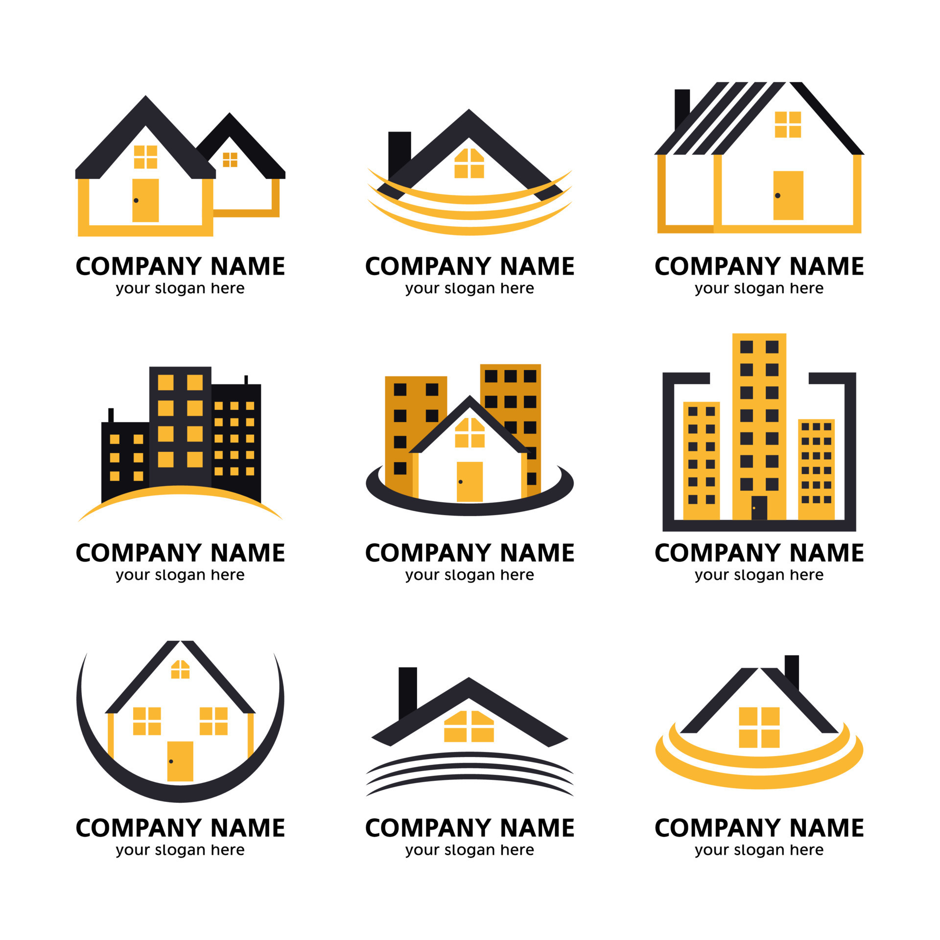
Here's a short list of some original name ideas to inspire you:
- BuildPro
- Constructo
- HomeCraft
- Renov8
- EcoBuild
- Structure Solutions
Construction Jobs and the Industry
The construction industry offers a wide range of roles and opportunities. From general contractors to estimators and project managers, there are various paths to explore. These jobs involve managing projects, estimating costs, and overseeing the entire building process. It's a dynamic industry with a lot of growth potential.
When it comes to salaries, it depends on the role, experience, and location. Construction jobs can offer competitive wages, and with the right skills and expertise, you can build a successful career. Many opportunities are available in cities like Houston, Atlanta, and San Francisco, where the construction industry is thriving.
Costs and Quotes: A Practical Guide
Understanding costs is essential when it comes to construction. The price of a project can vary greatly depending on factors like size, materials, and labor costs. It's always a good idea to get multiple quotes to compare and ensure you're getting a fair deal.
When comparing quotes, look beyond the price. Consider the scope of work, the company's reputation, and their experience. A lower price might not always be the best option if it means cutting corners or using lower-quality materials. Ask for references and check their previous work to get a sense of their quality and reliability.
Data and Tools: Behind the Scenes
In the construction industry, tools like RSMeans provide valuable data and cost estimates. These resources help professionals make informed decisions and plan projects effectively. RSMeans, for example, offers cost databases and escalation tools to account for potential price changes. It's a useful resource for contractors and estimators.
Wrapping Up
So, there you have it! Names for construction might seem like a simple phrase, but it covers a lot of ground. From naming your business to understanding the industry and its costs, there's a lot to consider. I hope this has given you some insights and inspired you to explore further. Remember, the construction industry is full of opportunities, and a great name can be your first step towards success.
Related: Create a 1-100 chart in Excel using data ranges
A 1-100 chart is a simple way to show numbers from one to one hundred in Excel. This post shows how to create it quickly using Excel fill series and a bar chart.
You can use the auto‑fill handle to generate the numbers, then turn the range into a chart with a few clicks. The exact steps can vary a bit depending on your Excel version, but the core idea stays the same.
Excel online guide: Create a 1‑100 chart with fill series and a bar chart
If you need a quick visual of the numbers from one to one hundred, a 1-100 chart is the simplest solution in Excel. You can generate the numbers automatically and turn them into a bar chart without any coding.
Start by using Excel auto fill numbers to populate a column with the sequence 1, 2, 3… up to 100. Select the filled range, then insert a bar chart to see each value as a bar.
The process works the same in recent versions such as Microsoft 365 Excel, Excel 2019, and Excel for the web, so you don’t need to worry about version differences.
Data range setup: What must be true first
Before you begin, make sure Excel is not in protected view and that the worksheet is not protected, otherwise fill commands will be disabled.
A clear range helps Excel data visualization tools work correctly. If you are on a corporate account, confirm that macros or add‑ins are not blocked by policy.
If you are using Excel on the web, ensure you have edit permissions for the file; a read‑only view will prevent the fill handle from working.
If you convert the filled range into an Excel table (Ctrl+T), the fill handle will automatically extend when you add new rows, and the chart will reference the entire table without manual range updates.
Fill series steps: How to generate numbers and build the chart
Follow these steps to create the numbers and the chart in a few minutes.
- Select cell A1 and type 1, then click the fill handle (small square at the corner) and drag down while holding the left mouse button to extend the series.
- Release the mouse and choose Fill Series from the AutoFill options that appear; this tells Excel to continue the numeric sequence.
- With the column selected, go to the Insert tab and choose 2-D Column from the Charts group to create a bar chart based on the data.
- Excel will place the chart on the sheet; click the chart to select it and use the Chart Design tab to adjust titles and axis labels if needed.
- If you want the chart to reflect the full 1-100 chart, make sure the data range includes cell A100; you can resize the selected area manually or let Excel auto‑detect the range.
- To improve readability, add a chart title like “Numbers 1‑100” and label the vertical axis as “Value”.
- Finally, save the workbook; the chart will update automatically if you later extend the fill series beyond 100.
Chart design basics: Why it may not work and what to check
Sometimes the chart appears blank, shows wrong values, or the fill series stops early; checking a few items usually fixes it.
- Make sure the fill handle was dragged correctly and the AutoFill option selected; without it Excel treats the numbers as plain text.
- Verify that the cells are formatted as General or Number; a custom format that hides values can cause the chart to be empty.
- Check that the chart’s data source range matches the filled column; a mismatched range can show only part of the sequence.
- Ensure the workbook is not in read‑only mode and that you have edit permission; otherwise Excel won’t update the chart.
After making any corrections, save the file and reopen it to confirm the chart displays the full sequence; a fresh open often resolves display glitches.
Axis labels adjust: A safer way to avoid problems next time
A more robust method is to create an Excel table for the numbers; when you add a new row, the table expands and the chart updates automatically.
You can also define a named range that uses the OFFSET function to grow as you fill, then base the chart on that named range instead of a fixed address.
If you prefer not to use a table, generate the numbers with a simple formula such as =ROW()-ROW($A$1)+1 in each cell; the chart will still reflect the 1-100 chart as long as the formula fills down.
Finally, keep axis labels simple and avoid merging cells; merged cells can interfere with chart selection and cause unexpected behavior.
Another option is to use a sparkline in a cell next to the numbers; it provides a compact visual of the trend without taking up sheet space, and it updates automatically as you fill.
Quick note: the menu names can look a bit different depending on your version of Excel, so don’t be surprised if something shows up in a different spot.
If you found this helpful, feel free to browse the other Microsoft Office guides on the site whenever you need a quick tip or a fix.
Related: how to create pivot chart Easy guide for Excel users
I've been working with spreadsheets for a while now, and one of the most useful skills I've learned is how to create pivot charts. It's a game-changer for visualizing data and making sense of complex information. So, let's dive into the process and see how we can make our data pop with these dynamic charts!
Setting Up Your Data for Success
When it comes to creating pivot charts, the first step is ensuring your data is structured properly. Think of your spreadsheet as a house; the columns are the rooms, and the rows are the items within each room. So, before we start, let's tidy up our data: make sure your columns have clear, concise headers, and your rows are consistent and organized. This step is crucial because it lays the foundation for an accurate and effective pivot chart.
Now, let's talk about the tools Excel provides to make this process smoother. Excel has some fantastic built-in features to help with data manipulation and formatting. For instance, you can use the XLOOKUP formula to quickly find and retrieve specific data points, or the IF function to create conditional rules for your data. These formulas are your friends and can save you a lot of time and effort, especially when dealing with large datasets.
Building Your Pivot Chart
Once your data is shipshape, it's time to build your pivot chart. Excel makes this process pretty straightforward. Go to the Insert tab and select PivotChart. From here, you'll be prompted to choose the data range you want to include in your chart. Excel will then display a new window where you can customize your chart's layout.
This is where the magic happens! You can drag and drop fields to create rows, columns, and even filters for your chart. For example, if you have a dataset with sales data, you could drag the "Product" field to the Rows area, and the "Sales Amount" field to the Values area. This will create a chart that shows the sales performance of each product.
Customizing and Refining
Now that you have your basic pivot chart, it's time to add some polish. Excel offers a range of customization options to make your chart truly shine. You can change the chart type, add titles and labels, and even apply conditional formatting to highlight specific data points. For instance, you could use conditional formatting to highlight cells with sales above a certain threshold, making it easy to identify top-performing products at a glance.
Another useful feature is the ability to create drop-down lists in your pivot chart. This allows you to quickly filter your data by selecting different options from a drop-down menu. It's a great way to make your chart more interactive and user-friendly.
Final Thoughts
So, there you have it! Creating pivot charts in Excel is a powerful way to visualize and analyze your data. It might seem a bit daunting at first, but with a bit of practice and familiarity with Excel's tools, you'll be creating dynamic charts in no time.
Next time you open a spreadsheet, why not give it a go? You might just discover a whole new way to understand and present your data.