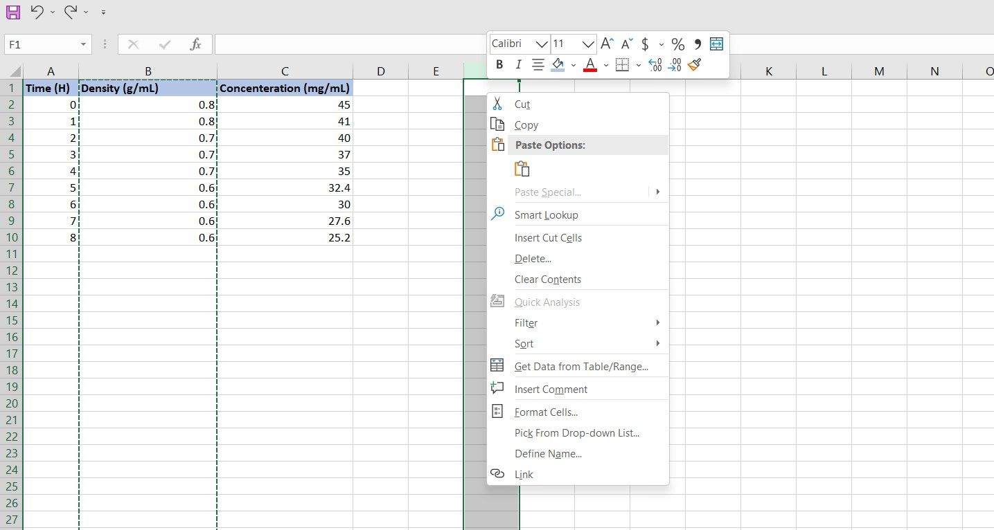



Rearrange columns for better analysis
If you’re working with a dataset that’s out of order, moving columns is a quick fix. Analysts and project managers benefit most here, especially when dealing with logs or trackers. For example, if you’ve got a sheet tracking tasks with columns like "Priority," "Due Date," and "Status," you might want "Status" front and center for a quick glance.
Set up your sheet with clear headers in row 1 and data starting in row 2. Keep related columns together—like grouping all date fields or all numerical values. This makes it easier to apply filters or sort later. If you’re using a table (Ctrl+T), moving columns within it updates any related formulas automatically.
Here’s a sample task tracker:
| Task ID | Priority | Due Date | Status | Hours Spent |
|---|---|---|---|---|
| 001 | High | 2023-10-15 | Completed | 8 |
| 002 | Medium | 2023-10-20 | In Progress | 4 |
| 003 | Low | 2023-10-25 | Pending | 0 |
To count completed tasks, use =COUNTIFS(Status, "Completed"). This formula returns 1 in this case, since only one task is marked as done.
A common mistake here is merging cells for headers, which breaks the table structure. Always keep headers in a single row and use Center Across Selection from the Alignment tab instead.
Drag and drop with formulas intact
Moving columns with formulas requires a bit of care. If you’ve got a column calculating totals, like =B2C2 for "Total Cost," dragging the column won’t break the formula—Excel updates references automatically. This works best when your sheet uses relative references.
Start by setting up a simple invoice tracker with columns like "Item," "Price," and "Quantity." Add a "Total" column with the formula above. If you move the "Quantity" column, the formula adjusts to =D2E2 if it’s now in column D.
| Item | Price | Quantity | Total |
|---|---|---|---|
| Widget | 10 | 5 | =B2C2 |
| Gadget | 20 | 3 | =B3C3 |
To avoid errors, use =IFERROR(B2*C2, "N/A") in the Total column. This catches any division by zero or missing values, returning "N/A" instead of an error.
One mistake to avoid is hard-coding values. If you type "5" directly into a cell instead of referencing another cell, moving columns won’t update it. Always use cell references for dynamic data.
Use tables for smarter column management
Converting your data range into a table (Ctrl+T) makes moving columns even smoother. Tables automatically adjust formulas and formatting, so you don’t have to worry about breaking anything.
Tables are ideal for logs or checklists where data grows over time. For instance, a project log with columns like "Date," "Task," and "Notes" can be rearranged without messing up filters or totals.
Here’s a sample project log table:
| Date | Task | Notes | Hours |
|---|---|---|---|
| 2023-10-01 | Client Meeting | Follow-up needed | 2 |
| 2023-10-02 | Draft Proposal | Waiting on feedback | 4 |
To sum hours, use =SUM(Table1[Hours]). If you move the "Hours" column, the formula still works because tables use structured references.
A common pitfall is forgetting to expand the table when adding new columns. Always click the table, go to Table Design > Resize Table, and update the range to include new data.
Fix broken references after moving
Even with careful planning, moving columns can sometimes break formulas. If you’ve got a VLOOKUP or XLOOKUP referencing a column you moved, you’ll need to update the formula manually.
For example, if your lookup formula references column C but you moved it to column E, change =XLOOKUP(A2, C:C, D:D) to =XLOOKUP(A2, E:E, F:F).
| ID | Name | Department | Manager |
|---|---|---|---|
| 1 | John | Sales | =XLOOKUP(C2, E:E, F:F) |
| 2 | Jane | Marketing | =XLOOKUP(C3, E:E, F:F) |
To prevent this, use named ranges or tables. Go to Formulas > Define Name, select the range, and give it a name like "Departments." Then use =XLOOKUP(A2, Departments, Managers)—this stays intact even if columns move.
One mistake is not checking for numbers stored as text. If a column with numerical data is formatted as text, formulas might not work after moving. Use Data > Text to Columns to convert it back to numbers.
Try moving a column in your own sheet and adding a conditional formatting rule to highlight values above a certain threshold. It’s a quick way to see how changes affect your data.