
Rainbow Dash Coloring Pages Overview
Many folks get tripped up by thinking a duct sizing chart is some kind of complex, mysterious tool, but it's actually a straightforward, handy reference. It's like a map to help you navigate the world of ductwork dimensions.
The chart provides a visual guide, often with easy-to-read tables, to ensure you select the right size duct for your HVAC system. While the values might vary slightly depending on your region or the specific standards you follow, the duct sizing chart is a reliable starting point, offering a simple, quick solution to a potentially confusing task.
Duct Sizing: Understanding the Chart
The duct sizing chart is your practical guide to selecting the right size ducts for your HVAC system. It's a simple yet effective tool that helps you match the duct dimensions to your specific needs, ensuring efficient airflow and a comfortable indoor environment.
Key Details and Categories
Before diving into the chart, it's essential to understand the basic units and categories. Duct sizes are typically measured in inches and represented by rectangular dimensions, such as 8x12 or 10x14. These dimensions refer to the height and width of the duct, respectively. The chart provides a range of standard sizes, covering various common duct types. You'll find sizes from small, like 4x6, to larger ones, such as 20x24, catering to different HVAC system requirements.
Interpreting the Chart: A Step-by-Step Guide
Using the duct sizing chart is straightforward. First, identify the type of duct you need, whether it's for supply, return, or exhaust airflow. Then, locate the relevant section on the chart. Each section will provide a range of sizes, along with their corresponding dimensions. For example, you might see a column with sizes like 10, 12, and 14, indicating the width, and a row with heights like 8, 10, and 12. Simply find the intersection of the desired width and height to get your duct size. Remember, the chart offers a standard range, so you may need to adjust slightly based on your specific system and installation constraints.
Variations and Differences
While the duct sizing chart provides a solid foundation, variations can occur due to several factors. Different standards and regions may have slightly different sizing guidelines, so it's crucial to refer to the appropriate standard for your location. Additionally, the type of HVAC system and its unique requirements can influence duct size. For instance, high-efficiency systems might need larger ducts to handle increased airflow. Installation constraints, such as limited space, can also impact the final duct size choice. It's always a good idea to consult with an HVAC professional to ensure you're selecting the right size for your specific situation.
In summary, the duct sizing chart is a valuable tool, offering a quick and easy way to determine duct sizes. By understanding the basic categories and following a simple step-by-step process, you can accurately select the right size ducts for your HVAC system. Remember, while the chart provides a great starting point, consulting experts and considering your unique circumstances is essential for optimal results.
Hey there, duct sizing enthusiasts! We hope this guide has given you a clear understanding of the process and the key factors to consider. Remember, while the basics remain the same, the exact values and specifications can differ slightly, so always double-check the relevant standards and sources for your specific project.
Consider bookmarking this page for future reference; it's a handy tool to have at your fingertips when you're in the middle of a project and need a quick reminder. We've got more practical guides like this one, so feel free to explore and discover other helpful resources. Happy sizing!
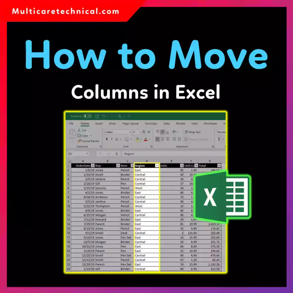
Related: how to move excel columns easy step by step guide
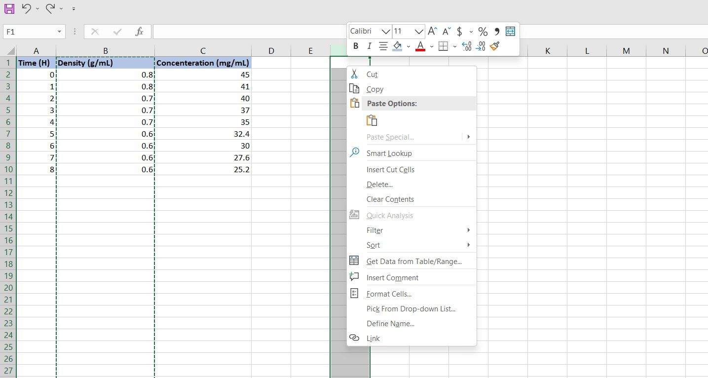
How to move Excel columns can save you a lot of time when rearranging data. Imagine you’ve got a sheet with sales data, but the "Region" column is stuck between "Product" and "Quantity," making it hard to analyze trends. Instead of copying and pasting everything, you can simply drag the column header to its new spot. It’s faster and keeps your formulas intact.
Moving columns isn’t just about aesthetics—it’s about making your data easier to work with. Whether you’re prepping a report or cleaning up a tracker, knowing how to move Excel columns ensures your sheet stays organized. Plus, it’s a skill that pairs well with other Excel tricks, like using tables or conditional formatting, to keep everything tidy.
Rearrange columns for better analysis
If you’re working with a dataset that’s out of order, moving columns is a quick fix. Analysts and project managers benefit most here, especially when dealing with logs or trackers. For example, if you’ve got a sheet tracking tasks with columns like "Priority," "Due Date," and "Status," you might want "Status" front and center for a quick glance.
Set up your sheet with clear headers in row 1 and data starting in row 2. Keep related columns together—like grouping all date fields or all numerical values. This makes it easier to apply filters or sort later. If you’re using a table (Ctrl+T), moving columns within it updates any related formulas automatically.
Here’s a sample task tracker:
| Task ID | Priority | Due Date | Status | Hours Spent |
|---|---|---|---|---|
| 001 | High | 2023-10-15 | Completed | 8 |
| 002 | Medium | 2023-10-20 | In Progress | 4 |
| 003 | Low | 2023-10-25 | Pending | 0 |
To count completed tasks, use =COUNTIFS(Status, "Completed"). This formula returns 1 in this case, since only one task is marked as done.
A common mistake here is merging cells for headers, which breaks the table structure. Always keep headers in a single row and use Center Across Selection from the Alignment tab instead.
Drag and drop with formulas intact
Moving columns with formulas requires a bit of care. If you’ve got a column calculating totals, like =B2C2 for "Total Cost," dragging the column won’t break the formula—Excel updates references automatically. This works best when your sheet uses relative references.
Start by setting up a simple invoice tracker with columns like "Item," "Price," and "Quantity." Add a "Total" column with the formula above. If you move the "Quantity" column, the formula adjusts to =D2E2 if it’s now in column D.
| Item | Price | Quantity | Total |
|---|---|---|---|
| Widget | 10 | 5 | =B2C2 |
| Gadget | 20 | 3 | =B3C3 |
To avoid errors, use =IFERROR(B2*C2, "N/A") in the Total column. This catches any division by zero or missing values, returning "N/A" instead of an error.
One mistake to avoid is hard-coding values. If you type "5" directly into a cell instead of referencing another cell, moving columns won’t update it. Always use cell references for dynamic data.
Use tables for smarter column management
Converting your data range into a table (Ctrl+T) makes moving columns even smoother. Tables automatically adjust formulas and formatting, so you don’t have to worry about breaking anything.
Tables are ideal for logs or checklists where data grows over time. For instance, a project log with columns like "Date," "Task," and "Notes" can be rearranged without messing up filters or totals.
Here’s a sample project log table:
| Date | Task | Notes | Hours |
|---|---|---|---|
| 2023-10-01 | Client Meeting | Follow-up needed | 2 |
| 2023-10-02 | Draft Proposal | Waiting on feedback | 4 |
To sum hours, use =SUM(Table1[Hours]). If you move the "Hours" column, the formula still works because tables use structured references.
A common pitfall is forgetting to expand the table when adding new columns. Always click the table, go to Table Design > Resize Table, and update the range to include new data.
Fix broken references after moving
Even with careful planning, moving columns can sometimes break formulas. If you’ve got a VLOOKUP or XLOOKUP referencing a column you moved, you’ll need to update the formula manually.
For example, if your lookup formula references column C but you moved it to column E, change =XLOOKUP(A2, C:C, D:D) to =XLOOKUP(A2, E:E, F:F).
| ID | Name | Department | Manager |
|---|---|---|---|
| 1 | John | Sales | =XLOOKUP(C2, E:E, F:F) |
| 2 | Jane | Marketing | =XLOOKUP(C3, E:E, F:F) |
To prevent this, use named ranges or tables. Go to Formulas > Define Name, select the range, and give it a name like "Departments." Then use =XLOOKUP(A2, Departments, Managers)—this stays intact even if columns move.
One mistake is not checking for numbers stored as text. If a column with numerical data is formatted as text, formulas might not work after moving. Use Data > Text to Columns to convert it back to numbers.
Try moving a column in your own sheet and adding a conditional formatting rule to highlight values above a certain threshold. It’s a quick way to see how changes affect your data.
Related: Create a 1-100 chart in Excel using data ranges
A 1-100 chart is a simple way to show numbers from one to one hundred in Excel. This post shows how to create it quickly using Excel fill series and a bar chart.
You can use the auto‑fill handle to generate the numbers, then turn the range into a chart with a few clicks. The exact steps can vary a bit depending on your Excel version, but the core idea stays the same.
Excel online guide: Create a 1‑100 chart with fill series and a bar chart
If you need a quick visual of the numbers from one to one hundred, a 1-100 chart is the simplest solution in Excel. You can generate the numbers automatically and turn them into a bar chart without any coding.
Start by using Excel auto fill numbers to populate a column with the sequence 1, 2, 3… up to 100. Select the filled range, then insert a bar chart to see each value as a bar.
The process works the same in recent versions such as Microsoft 365 Excel, Excel 2019, and Excel for the web, so you don’t need to worry about version differences.
Data range setup: What must be true first
Before you begin, make sure Excel is not in protected view and that the worksheet is not protected, otherwise fill commands will be disabled.
A clear range helps Excel data visualization tools work correctly. If you are on a corporate account, confirm that macros or add‑ins are not blocked by policy.
If you are using Excel on the web, ensure you have edit permissions for the file; a read‑only view will prevent the fill handle from working.
If you convert the filled range into an Excel table (Ctrl+T), the fill handle will automatically extend when you add new rows, and the chart will reference the entire table without manual range updates.
Fill series steps: How to generate numbers and build the chart
Follow these steps to create the numbers and the chart in a few minutes.
- Select cell A1 and type 1, then click the fill handle (small square at the corner) and drag down while holding the left mouse button to extend the series.
- Release the mouse and choose Fill Series from the AutoFill options that appear; this tells Excel to continue the numeric sequence.
- With the column selected, go to the Insert tab and choose 2-D Column from the Charts group to create a bar chart based on the data.
- Excel will place the chart on the sheet; click the chart to select it and use the Chart Design tab to adjust titles and axis labels if needed.
- If you want the chart to reflect the full 1-100 chart, make sure the data range includes cell A100; you can resize the selected area manually or let Excel auto‑detect the range.
- To improve readability, add a chart title like “Numbers 1‑100” and label the vertical axis as “Value”.
- Finally, save the workbook; the chart will update automatically if you later extend the fill series beyond 100.
Chart design basics: Why it may not work and what to check
Sometimes the chart appears blank, shows wrong values, or the fill series stops early; checking a few items usually fixes it.
- Make sure the fill handle was dragged correctly and the AutoFill option selected; without it Excel treats the numbers as plain text.
- Verify that the cells are formatted as General or Number; a custom format that hides values can cause the chart to be empty.
- Check that the chart’s data source range matches the filled column; a mismatched range can show only part of the sequence.
- Ensure the workbook is not in read‑only mode and that you have edit permission; otherwise Excel won’t update the chart.
After making any corrections, save the file and reopen it to confirm the chart displays the full sequence; a fresh open often resolves display glitches.
Axis labels adjust: A safer way to avoid problems next time
A more robust method is to create an Excel table for the numbers; when you add a new row, the table expands and the chart updates automatically.
You can also define a named range that uses the OFFSET function to grow as you fill, then base the chart on that named range instead of a fixed address.
If you prefer not to use a table, generate the numbers with a simple formula such as =ROW()-ROW($A$1)+1 in each cell; the chart will still reflect the 1-100 chart as long as the formula fills down.
Finally, keep axis labels simple and avoid merging cells; merged cells can interfere with chart selection and cause unexpected behavior.
Another option is to use a sparkline in a cell next to the numbers; it provides a compact visual of the trend without taking up sheet space, and it updates automatically as you fill.
Quick note: the menu names can look a bit different depending on your version of Excel, so don’t be surprised if something shows up in a different spot.
If you found this helpful, feel free to browse the other Microsoft Office guides on the site whenever you need a quick tip or a fix.